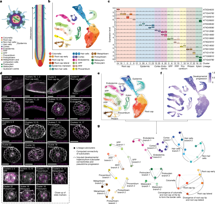
Plant material and growth conditionsSeeds from wild-type A. thaliana ecotypes (Col-0, Ws-2, Cvi-0, c24 and Ler) or the mutants aba2-3 (Col-0 background, ABRC stock number CS3834), pyl11458 (Col-0 background, ABRC stock number CS72390) and scr-3 (Col-0 background, NASC stock code N3997) were sterilized and densely sown in rows on 1× (or 0.5× when testing the effect of nutrient concentration) MS basal medium with vitamins (Austratec) on 0.9% agar plates supplemented with 1% sucrose (pH 5.7) and stratified in the dark at 4 °C for 2 days. Plates were subsequently grown in long day conditions (16 h of light, 8 h of dark) at 22 °C. At 6–7 days after germination (d.a.g.), root tips (up to around 3 mm) were collected for protoplast isolation using sharp tweezers. For all experiments, seedlings were grown under identical conditions and collected at the same time of day. For all comparative experiments (MS concentrations or water-deficit), seedlings from the different conditions were sterilized, plated, grown and harvested simultaneously.Hard-agar model of droughtFor the hard-agar water-deficit assay, seedlings were grown on 0.5× MS medium under control conditions (100% water content) or on 0.5× MS medium with the water content reduced to 50% or 20% of the control level (corresponding to 1× MS with 1.8% agar and 2.5× MS with 4.5% agar, respectively). Seedlings were otherwise grown and collected under the same conditions as described above.Roots growing through agarIn standard plate assays, roots are grown along the agar surface and are simultaneously exposed to two microenvironments: air on one side and agar on the other. To test whether this heterogeneous exposure influences the formation of the ERS described in this study, roots were instead grown entirely in the agar to provide a homogeneous environment. To do so, square plates were filled with 1× MS medium as described above. After solidification, the medium was cut in half with a razor blade under sterile conditions. Seeds were placed at the top edge of the cut agar and plates were positioned vertically in the growth chamber, allowing cotyledons to develop at the surface while roots penetrated and grew through the agar. Root tips were collected with fine tweezers at the same developmental stage and time point as described above.Protoplast isolation and scRNA-seqRoot tips were placed in 15 ml protoplasting solution45 (1.25% w/v cellulase, 0.3% w/v macerozyme, 0.4 M d-mannitol, 20 mM MES (pH 5.7), 20 mM KCl, 10 mM CaCl2, 0.5% w/v BSA and 5 mM β-mercaptoethanol in ultrapure water) and incubated at room temperature for 1 h on a tube rotator. The solution was subsequently filtered through a 70 μm strainer and a 40 μm cell strainer (Falcon) to separate protoplasts from undissociated tissue. Cells were centrifuged for 5 min at 500g in a swinging bucket centrifuge. The pellet was resuspended in 15 ml protoplast resuspension buffer (0.4 M d-mannitol, 20 mM MES (pH 5.7), 20 mM KCl, 10 mM CaCl2 and 0.5% w/v BSA in ultrapure water) and centrifuged at 500g for 5 min. Cells were resuspended in the protoplast resuspension buffer and filtered through a 35 μm cell strainer Snap Cap (Falcon). When preparations involved two Arabidopsis ecotypes, protoplasts from each background were mixed in equal proportions. The final concentration was adjusted to 900–1,200 cells per μl and barcoded using a Chromium Controller (10x Genomics). Libraries were generated with reagents from a Single Cell Gene Expression kit (10x Genomics, Single Cell 3′ Library kit) according to the manufacturer’s instructions. Libraries were sequenced either on an Illumina NextSeq 500 or a NovaSeq 6000, following recommendations of 10x Genomics.PreprocessingAll the data preprocessing steps are summarized in Supplementary Fig. 1.MappingReads were mapped using the 10x Genomics CellRanger pipeline (v.7.1.0) to the TAIR10 Arabidopsis genome with the –expect-cells=10000 parameter.If the cell preparation contained a mix of two ecotypes, reads were mapped to a version of the Arabidopsis (TAIR10) genome with ambiguous base codes placed at single-nucleotide polymorphism (SNP) positions for the genotypes sequenced, as identified by the Arabidopsis 1001 genomes project46.Low-quality cell filteringRecent versions of CellRanger identify substantially more cells than earlier releases. This enables the detection of low-UMI root cap cells (which were discarded in earlier releases), but also results in the identification of more cells than expected based on cell loading in the assay. Many of these seem to be low-UMI, low-quality cells, which are probably derived from damaged protoplasts that nonetheless pass the CellRanger threshold. To identify and remove such cells, we developed a filtering approach based on clustering CellRanger-called ‘cell’ barcodes together with barcodes classified as background. The method was applied independently to each library and manually adjusted, which enabled the proportion of filtered cells to vary according to the intrinsic quality of each preparation. The procedure (illustrated in Supplementary Fig. 1) is described below.A Seurat (v.5.0.0)47 object was created from the N barcodes identified as cells by CellRanger, excluding genes expressed in fewer than three cells. Data were log-normalized and scaled. Highly variable genes (HVGs) were identified using FindVariableFeatures (nfeatures=15,000). Genes affected by protoplast isolation (see the section ‘Identification of genes affected by protoplast isolation’), as well as mitochondrial and chloroplastic genes, were excluded from the HVG set. The first 40 principal components were used for UMAP dimensionality reduction and clustering. Major root cell types (root cap, epidermis, cortex, endodermis, pericycle, phloem, xylem and procambium) were annotated.The following steps were applied to each cell type individually:
A new Seurat object was created containing the ‘cell type’ cells and the first top N barcodes (ranked by UMI content) that were classified as background by CellRanger. The object was processed as above, with the exception that FindVariableFeatures was run with the parameter nfeatures=5000 and that the first 20 principal components were used for UMAP and cell clustering.
The object was subsetted to retain only the cluster (or clusters) containing the ‘cell type’ cells, which typically also includes some background barcodes. This subsetted object was then re-processed as in the previous step.
In this subset, background barcodes typically form distinct clusters, often together with low-quality cells of the given type. All cells clustering with background were considered more similar to background than to high-quality cells and were reclassified as background and discarded.
Using this approach, between 8 and 30% of CellRanger-identified cells were typically removed. Preparations processed using 10x Genomics NextGem chemistry tended to generate a higher proportion of discarded cells.Doublet identificationDoublets were identified using scDblFinder48,49 following the recommendations of the Single-cell Best Practices guide (www.sc-best-practices.org). The analysis was performed on the Seurat object obtained after cell filtering, with the parameters artificialDoublets=25000, dims=30, dbr.sd=1 and propRandom=1. All cells identified as doublets were subsequently removed from the dataset.Cell genotypingAfter doublet removal, preparations composed of a mix of two Arabidopsis ecotypes were subjected to cell genotyping based on SNPs. SNP UMIs were counted per cell using the countsnps command in the sctools package (https://github.com/timoast/sctools). To separate the two ecotype populations, density-based clustering was performed on the SNP UMI counts for each ecotype using the dbscan50 package in R (Supplementary Fig. 1), with the eps and minPts parameters adjusted for each dataset. The few cells that did not cluster with either population were discarded.Data integrationEach condition included at least three replicates, except for the water-deficit experiments, which had two replicates each. Replicates were integrated using Seurat (v.5.0.0) to generate batch-corrected atlases. In brief, replicates were merged into a single Seurat object. HVGs were detected using the FindVariableFeatures function with nfeatures=25000. Genes affected by protoplasting, as well as mitochondrial and chloroplastic genes, were excluded from the HVG dataset. Data were scaled, and the first 50 principal components were computed using RunPCA. Replicates were then integrated using the anchor-based RPCA method in Seurat (v.5.0.0) with IntegrateLayers, using method=RPCAIntegration and dims=1:50.For the Col-0 reference atlas, the replicates RL650, RL970 and RL971, which exhibited the highest data complexity, were used as reference during integration with reference=1:3. The resulting 50-dimensional integrated RPCA reduction was used for UMAP and clustering.In some cases, after the integration step, a few diffuse groups of low-UMI cells could be identified associated with the epidermis and cortex lineages, which probably represent low-quality cells that had passed the initial filtering step. To remove these, separate ‘epidermis–root cap’ and ‘cortex’ objects were created, re-integrated and processed as described above. After removing the low-quality cells, the atlas was re-processed with RPCA integration, and the first 45 dimensions were used for UMAP and clustering.In other cases beyond the Col-0 atlas, small clusters of low-quality cells were also removed; see the integration scripts for further details.Identification of genes affected by protoplast isolationPlants were prepared as for scRNA-seq, as described above. Four replicates each of dissociated and non-dissociated root tips were compared. For dissociated samples, root tips were placed in the protoplasting solution for 1 h at room temperature, as for scRNA-seq. After this incubation step, samples were centrifuged for 5 min at 500g, the supernatant was removed and the tissue samples were snap-frozen in liquid nitrogen and ground into a powder. For non-dissociated samples, root tips were collected and directly snap-frozen and ground into powder in liquid nitrogen. Bulk RNA-seq libraries were generated using a TruSeq stranded mRNA kit (Illumina). Bulk RNA-seq libraries were sequenced on an Illumina HiSeq 1500 (single end, 101 cycles). RNA-seq read quality was assessed using FastQC and MultiQC51,52. RNA-seq reads were trimmed using Trimmomatic (v.0.36) with the following parameters: ILLUMINACLIP:TruSeq3-SE.fa:2:30:10 LEADING:3 TRAILING:3 SLIDINGWINDOW:4:15 MINLEN:36 (ref. 53). Reads were aligned to the TAIR10 genome using STAR54 with the following parameters: –alignIntronMax 5000, –alignIntronMin 10, –readFilesCommand zcat, –quantMode GeneCounts, –outSAMtype BAM SortedByCoordinate. Differentially expressed genes resulting from the cell dissociation step were identified using the DESeq2 R package55, with a Benjamini–Hochberg adjusted P 2 fold change in expression of >2. This experiment was repeated twice, and genes that were identified as differentially expressed in both experiments were taken as the set of genes affected by protoplast isolation.Whole-mount in situ HCRProbe designCandidate cluster markers for our reference atlas were generated using the FindAllMarkers function in Seurat, with the only.pos = TRUE parameter. To select the best target genes, cluster markers were filtered on the basis of the following criteria: the gene should be detected almost only in the cluster (or clusters) it is enriched in; and the gene should have a large portion of its coding sequence that does not share homology with other Arabidopsis genes, which will enable the design of highly specific probes for these sequences. Split probes for our target genes were designed and synthesized by Molecular Instruments (www.molecularinstruments.com).Sample fixation and dehydrationExperiments were performed as previously described56. Roots were collected at 6 d.a.g., as for scRNA-seq, and immediately placed in FAA (7.4% formaldehyde, 5% acetic acid and 50% ethanol in ultrapure water) for 1 h at room temperature. Samples were then dehydrated in successive 10 min washes at room temperature: once in 70% ethanol, once in 90% ethanol and twice in 100% ethanol. Samples were washed twice in 100% methanol and left in the second wash at −20 °C overnight (or up to a few weeks).Permeabilization and protease digestionRoots were rehydrated in a series of 5 min washes at room temperature in 75%, 50%, 25% methanol and in DPBS-T (0.1% Tween 20 in DPBS) and incubated in 1× cell wall digestion solution (10× stock: 250 mg macerozyme, 250 mg cellulase, 125 mg pectolyase and 375 mg pectinase in 50 ml ultrapure water) in DPBS-T for 5 min. After a wash in DPBS-T, samples were fixed in 10% (v/v) formaldehyde (37% solution, Sigma-Aldrich) in DPBS-T for 15 min at room temperature and washed twice in DPBS-T. Roots were incubated in 1 ml proteinase K buffer (0.1 M Tris-HCl (pH 8) and 50 mM EDTA (pH 8) in ultrapure water) with 8 μl proteinase K (10 mg ml–1) for 15 min at 37 °C. After two washes in DPBS-T, samples were fixed in 10% (v/v) formaldehyde (37% solution, Sigma-Aldrich) in DPBS-T for 15 min at room temperature and washed twice in DPBS-T.Probe hybridization and amplificationWe followed the third-generation in situ HCR procedure developed by Molecular Instruments, and as previously described10, but the dextran sulfate used in the amplification buffer had to be replaced by a low-molecular-weight dextran sulfate to preserve the root structure. Roots were pre-hybridized in the 30% probe hybridization buffer for 30 min at 37 °C, then placed in the probe solution (2–3 μl of probe mixture in 500 μl of 30% probe hybridization buffer) and incubated at 37 °C overnight.Samples were washed twice in the 30% probe wash buffer for 30 min at 37 °C, then washed twice in 5× SSCT (5× SSC and 0.1% Tween 20 in ultrapure water) for 10 min at room temperature. Samples were placed in the amplification buffer for 30 min at room temperature. In the meantime, fluorescently labelled hairpins were prepared by snap-cooling 10 μl of 3 μM stock in hairpin storage buffer (heat at 95 °C for 90 s in a thermocycler and cool to room temperature in the dark for 30 min). We predominantly used HCR amplifiers coupled to Alexa 647 fluorophores in this study, with Alexa 488-coupled amplifiers used for experiments targeting two genes simultaneously. The hairpin solution was prepared by adding the snap-cooled hairpins to 500 μl amplification buffer. Samples were placed in the hairpin solution and incubated overnight at room temperature in the dark. They were subsequently washed 3 times in 5× SSCT for 20 min at room temperature.Clearing, cell wall staining and sample mountingSamples were incubated in ClearSee11 in the dark for 3 days.Cell walls were stained by incubating samples in 1 ml ClearSee and 2 μl calcofluor solution (50 mg ml–1 in DMSO) for 2 h in the dark. Samples were washed in ClearSee for 1 h, in the dark, and mounted in ClearSee in a chamber made with a square coverslip and double-sided tape. The chamber was sealed using top coat nail polish, and samples were imaged on the same day.ImagingMounted roots were imaged using a Nikon Ti-E inverted motorized microscope with a Nikon A1Si spectral detector confocal system or a Nikon A1RMP confocal microscope, controlled by NIS-Elements software, and a ×60 water-immersion objective. Calcofluor white and the Alex 488- and the Alexa 647-coupled amplifiers were excited at 405 nm, 488 nm and 640 nm, respectively. Seven to eight images were taken per root along the differentiation axis. Images were processed using Fiji57. Images of the same roots were stitched using the Grid/Collection stitching plugin58, and the brightness and contrast were adjusted for each image based on the signal detected. Optical sections were generated using the Orthogonal Views method in Fiji.Cell annotationAll datasets other than the Col-0 atlas were annotated using the Col-0 atlas as the reference. Anchors between the reference atlas and the other datasets were identified using FindTransferAnchors in Seurat (v.5), specifying the Col-0 RPCA-integrated data as the reference assay. TransferData in Seurat (v.5) was then used to calculate, for each cell, a prediction score for every identity, based on the identified anchors and the atlas annotations. Each cell was assigned the identity with the highest prediction score.Cell cycle annotationWe used the CellCycleScoring function in Seurat to assign a cell cycle score to each cell of our reference atlas based on the expression of S phase marker genes (E2Fc (also known as AT1G47870), E2Fb (AT5G22220), DPa (also known as AT5G02470), CDKG;2 (also known as AT1G67580), E2Fa (also known as AT2G36010), DPb (also known as AT5G03415), CYCA3;1 (also known as AT5G43080), CYCA3;2 (also known as AT1G47210), KRP5 (also known as AT3G24810), KRP2 (also known as AT3G50630), KRP6 (also known as AT3G19150), KRP3 (also known as AT5G48820), WEE (also known as AT1G02970), KRP4 (also known as AT2G32710), CYCD4;2 (also known as AT5G10440)) and of G2/M phase marker genes (CYCB1;1 (also known as AT4G37490), CYCB2;1 (also known as AT2G17620), CDKB2;2 (also known as AT1G20930), CYCB3;1 (also known as AT1G16330), CYCA2;2 (also known as AT5G11300), CYCA2;4 (also known as AT1G80370), CYCA1;1 (also known as AT1G44110), CYCA2;1 (also known as AT5G25380), CDKD;1 (also known as AT1G73690), CDKB2;1 (also known as AT1G76540), CKS2 (also known as AT2G27970), CYCB1;2 (also known as AT5G06150), CYCD3;1 (also known as AT4G34160), CCS52B (also known as AT5G13840), CYCA2;3 (also known as AT1G15570), CCS52A2 (also known as AT4G11920), CYCB2;3 (also known as AT1G20610) and CYCB1;3 (also known as AT3G11520)) obtained from a previous study59. This score was used to provide a predicted classification of the cell cycle phase and to regress out cell cycle effects using vars.to.regress = c(“S.Score”, “G2M.Score”) in the ScaleData function. After regression, the top 50 principal components were calculated and the replicates were integrated again. UMAP dimensionality reduction was then performed, and cell identities were visualized in the embedding to confirm that both branches remained present.Pseudotime trajectory analysesPAGAThe Col-0 atlas was subsetted into nine lineage-specific objects: epidermis, root cap, cortex, endodermis, PPP, XPP, procambium, phloem and xylem. Each lineage dataset was then processed independently.Subclusters in each lineage were identified using FindNeighbors and FindClusters in Seurat (v.5), with the values of dims, k.param and resolution adapted to each lineage.For each lineage, a ‘root cell’ corresponding to t = 0 in the trajectory was defined, as required by the diffusion pseudotime analysis underlying the PAGA trajectory inference. In the case of the epidermis and root cap lineages, developmental progression is known to originate at their junction. Therefore, for the epidermal lineage, the root cell was defined as the cell with the lowest coordinate along the UMAP y axis. For the root cap lineage, the root cell was defined as the cell with the highest coordinate along the UMAP y axis. For all other lineages, for which such anatomical landmarks are less obvious, the root cell was defined as the cell with the highest meristematic score (see below).To perform trajectory inference, we used the SCP package60, which implements PAGA61,62,63 analysis directly in R, thereby avoiding conversion of Seurat objects to AnnData format to run scanpy63. Seurat v.5 assays were first converted to v.3 assays to enable SCP. Trajectories were inferred with the RunPAGA function, grouping cells by the subclusters defined above, with the following parameters: inear_reduction = “integrated.rpca”, nonlinear_reduction = “umap.rpca”, infer_pseudotime=TRUE, n_pcs and n_neighbours matching the values used for subclustering, and root_cell containing the barcode of the designated root cell. The trajectory topology was visualized with the PAGAPlot function, using reduction = “umap.rpca” and an edge_threshold adapted to each lineage. The pseudotime value assigned to each cell was then transferred to the metadata of the original Seurat (v.5) object.Meristematic score calculationThe diffusion pseudotime analysis required the identification of a cell that would serve as t = 0; that is, the starting point of each trajectory. To do so, we developed an approach for identifying the ‘most meristematic’ cell in each lineage.The epidermis is the only lineage for which the meristematic region can be unambiguously located based on both the topology of its clusters and the known biology of the tissue. It lies at the junction with the root cap, before differentiation into the two epidermal subtypes: hair cells and non-hair cells. This cluster was therefore designated as epidermis–meristem. To identify marker genes for this region, we ran the FindMarkers function on the subsetted Seurat object containing only epidermal clusters, with ident.1 = 5 (corresponding to the ‘epidermis–meristem’ cluster), only.pos=TRUE, and test.use = ‘t’. The resulting gene list was then used with the AddModuleScore function in Seurat (v.5) to assign a meristematic score to every cell in the atlas.We reasoned that at least a subset of the genes enriched in the epidermal meristem would also be enriched in meristematic regions of other lineages. Thus, the cell with the highest meristematic score in each lineage was taken to represent the most likely earliest developmental state and used as the root cell (t = 0) for pseudotime analysis.Monocle analysisMonocle 3 (v.1.3.7)64,65,66 was used as an alternative method to confirm the developmental trajectories obtained using PAGA. Our Col-0 atlas was converted to a cds object using SeuratWrappers (v.0.4.0) (https://github.com/satijalab/seurat-wrappers). Cells were clustered and partitioned with cluster_cells using resolution=0.0002, and trajectories were computed using learn_graph with learn_graph_control=list(minimal_branch_len=20)). As for the PAGA trajectories, root cells were defined as those with the highest meristematic score per lineage, and these were used in order_cells to assign a pseudotime to each cell in the trajectory. All plots were generated with plot_cells. Concordance between (scaled) Monocle and diffusion pseudotime assignments was assessed using Spearman’s correlation coefficients computed independently for each lineage.scVelo analysisRNA velocity analysis was performed using the dynamical model implemented in the R package velociraptor67 (v.1.10.0) (wrapping scVelo68) on a per-lineage basis. Spliced and unspliced count matrices were generated independently for each library from velocyto69 (v.0.17.17) loom files and merged after restricting to genes detected across all samples. Because the intronic signal in Arabidopsis scRNA-seq datasets is limited, only genes with sufficient spliced and unspliced coverage were retained for velocity inference (minimum 50 cells with unspliced counts and 300 total unspliced counts; minimum 50 cells with spliced counts and 1,000 total spliced counts globally across the dataset). The top 4,000 variable genes were identified independently for each lineage, and protoplasting-sensitive genes, mitochondrial genes and chloroplast genes were excluded before analysis. The final gene set used for velocity inference corresponded to the intersection between lineage variable features and genes passing global spliced or unspliced filtering criteria. For each lineage, a SingleCellExperiment object containing spliced, unspliced and total RNA counts was generated and analysed using the scVelo dynamical model with the RPCA integrated embedding used as the neighbourhood graph for kinetic inference. Root cells for latent time estimation were defined independently for each lineage as the top 1% of cells with the highest meristematic score. Given the relatively low proportion of unspliced reads in our dataset (about 3% median unspliced fraction), RNA velocity was used primarily as an orthogonal validation of trajectory structure rather than as the primary trajectory inference approach. Concordance between scVelo latent time and diffusion pseudotime was assessed using Spearman’s correlation coefficients computed independently for each lineage.Expression-level analysis of ERS-associated genesTo test whether the apparent absence of ERS-associated genes in ERS− cells could be explained by reduced transcript capture, we compared the expression behaviour of genes from ERS+-specific modules (modules 20 and 21) and modules expressed in both branches (modules 13 and 14) in the XPP lineage, the largest lineage exhibiting the ERS dichotomy. Average log-normalized expression was calculated independently in ERS+ and ERS− cells for each gene. To compare genes across a shared expression range, overlapping expression intervals between ERS+-specific and shared-module genes were defined using the 10–90th percentile range of average ERS+ expression for each group. A linear model describing the relationship between ERS+ and ERS− expression was then fitted using genes from modules expressed in both branches. Residual ERS− expression values (observed minus expected expression) were subsequently calculated for all genes relative to this model. Residual distributions were compared between ERS+-specific genes and genes expressed in both branches in the overlapping expression interval using a two-sided Wilcoxon rank-sum test. This analysis tested whether ERS+-specific genes exhibited systematically lower ERS− expression than expected based solely on their expression level in ERS+ cells.UMI downsamplingBecause the number of transcripts detected in branch 1 was systematically higher than in branch 2, we tested whether the observed branching events could result from coverage artefacts. To control for this factor, UMI counts were selectively downsampled in ERS+ cells to match the UMI distribution of ERS− cells in each cell type. Specifically, for each ERS+ cell, a target UMI count was assigned based on quantile matching to the corresponding ERS− cell-type distribution, and counts were downsampled using the downsampleMatrix function from DropletUtils70 (v1.20.0). ERS− cells were left unchanged. Three independent downsampled count matrices were generated using different random seeds. Each downsampled matrix was used to generate a new Seurat object, which was processed independently using the same workflow as the reference atlas, including log-normalization, variable feature selection, scaling, PCA and UMAP embedding. Protoplasting-sensitive genes, mitochondrial genes and chloroplast genes were excluded from the variable feature set before dimensionality reduction. A meristematic score was then calculated for each cell using the same gene set as in the reference atlas.Identification of gene co-expression modulesWe used hdWGCNA (v0.4.1)71,72,73 to identify modules of co-expressed genes across our Col-0 reference atlas. To determine the list of genes that would be used in the analysis, we first applied the SetupForWGCNA function to obtain all genes expressed in at least 10% of cells in at least one lineage. This list was intersected with the VariableFeatures of the atlas, which contains all genes detected in every replicate, excluding those affected by protoplast isolation as well as mitochondrial and chloroplastic genes. The resulting set of 12,923 genes was supplied to SetupForWGCNA with the parameter gene_select = “custom”.To reduce data sparsity before WGCNA, we generated metacells (aggregates of small groups of similar cells per biological sample) and their associated expression matrices, which served as inputs for the network analysis. Metacells were generated using the MetacellsByGroups function using group.by=c(“lineage”,“orig.ident”), reduction = “integrated.rpca”, ident.group = “lineage”, k = 20 and max_shared=5, followed by normalization with NormalizeMetacells.We then set up the expression dataset for consensus network analysis across all replicates using SetMultiExpr with multi.group.by = “orig.ident”. After determining the soft power threshold for each batch with the TestSoftPowersConsensus function, the consensus co-expression network was constructed using ConstructNetworkusing minModuleSize=30, consensus=TRUE and deepSplit=2.Module scores were computed using ModuleExprScore using n_genes = “all” and method = “Seurat”, and projected onto the atlas UMAP with ModuleFeaturePlot using features = “scores”.GO enrichment analysis for ERS-specific modulesGO enrichment analysis was performed on the gene sets from modules 20 and 21 using ShinyGO (v.0.82; https://bioinformatics.sdstate.edu/go/). The analysis was run with the GO Biological Process pathway database, an FDR cut-off value of 0.01 and the number of pathways to display set to 50. Pathways were ranked by fold enrichment, and the results were visualized as a hierarchical clustering tree.TF regulon analysisPutative TF target genes were inferred from the DAP-seq dataset17. The ‘Motifs in peaks (P ≤ 1 × 10⁻⁴)’ BED file (http://neomorph.salk.edu/dap_web/pages/browse_table_aj.php) was used as a DNA-binding database for the profiled TFs of the DAP-seq dataset.The 500 bp promoter coordinates for Arabidopsis genes were extracted using the promoters function in GenomicRanges74, genes(TxDb.Athaliana.BioMart.plantsmart28) as an annotation for Arabidopsis genes and the arguments upstream = 500, downstream = 50. For each TF, the binding coordinates were extracted from the Motif in Peaks.bed file and intersected with the promoter coordinates using the subsetByOverlaps function in GenomicRanges. Every gene that had a binding motif for the TF in the 500 bp region upstream of its transcription start site (TSS) was considered a putative target gene. For TFs that were not profiled in the DAP-seq studies but, according to the cisBP2 study18, have a strong similarity in their DNA-binding domains with another TF that was studied by DAP-seq, their target genes were considered to be the same as the TF profiled by DAP-seq.We then converted the TF target predictions into data to be processed with hdWGCNA. A sparse matrix was generated whereby rows are all genes in the dataset, columns are TFs with putative targets and values are set to 1 if the gene was a target of the TF and 0 otherwise. This was input into the Seurat object using the SetMotifMatrix function of hdWGCNA (v.0.4.1). The list of TFs and their target genes was set with SetMotifTargets, and a dataframe containing the target numbers was input with SetMotifs. Because we were interested in what drives the expression of co-expression modules in the dataset, we restricted the analysis to all genes that were assigned to a co-expression module as well as all TFs with target information. A network of TFs and target genes was built using ConstructTFNetwork, in which the XGBoost regression was used to evaluate how important each TF is for predicting each gene based on single-cell data72,75. The network was then pruned to keep only the strongest TF–gene connections. Specifically, we selected the top ten TFs above a regulatory score threshold as regulators for each gene, using the AssignTFRegulons function with strategy = “A”, reg_thresh=0.01 and n_tfs=10. A positive regulon score was then computed for each cell using RegulonScores, and the scaled average regulon score per cell identity was plotted using pheatmap76.Analysis of published single-cell and single-nucleus datasetsThree published Arabidopsis root single-cell datasets were used to verify that the ERS and associated ERS-specific genes described in this study are also present in other datasets7,8,16. For ref. 8, we directly used the processed Seurat object provided by the authors. For ref. 7, we reprocessed the raw fastq files using the same pre-processing steps as described for our Col-0 atlas. For ref. 16, we used the count matrices provided by the authors and performed batch integration.Once the final Seurat objects were generated, cells were annotated using our reference atlas following the same procedure described in the section ‘Cell annotation’ above. Cells were also projected onto the atlas UMAP embedding using the MapQuery function in Seurat (v.5.0.0). Co-expression gene modules were projected onto these datasets using the ProjectModules function in hdWGCNA (v.0.4.1), and module scores were calculated with ModuleExprScore using n_genes = “all” and method = “Seurat”.Label-transfer stability analysisTo assess the robustness of ERS assignments in external datasets, label transfer was repeated across a range of Seurat parameter settings using the integrated Col-0 atlas as reference. Specifically, projections were performed using 30, 40 or 50 principal components and k.anchor values of 5, 10 or 20, which generated nine parameter combinations in total. For each parameter set, transfer anchors were identified using FindTransferAnchors with the RPCA integrated embedding, and cell identities were assigned using TransferData. To focus analyses on cells robustly assigned to the ERS bifurcation, only cells classified as ERS+ or ERS− in the baseline parameter set (50 principal components, k.anchor = 5) were retained for downstream comparisons. Predicted identities were separated into cell-type and ERS-state components, and stability was assessed independently for both. Cell-type stability was quantified as the fraction of parameter sets in which each cell retained its baseline cell-type assignment, whereas ERS stability was calculated as the consistency of ERS+ and ERS− assignment in the baseline cell type across parameter sets. Global agreement between parameter sets was further quantified using pairwise adjusted rand index (ARI) comparisons across all transferred labels. Furthermore, the proportion of ERS+ cells in each cell type, the fraction of cells retaining their baseline cell type assignment and the frequency of ERS state switching across parameter sets were calculated independently for each external dataset.Analysis of a previously published snATAC-seq datasetThe fragment files generated with Cell Ranger ATAC (v.1.2) and mapped to TAIR10/Araport11 reference were obtained from a previous study16, imported to snapatac2 (v.2.6.4) and paired-insertions calculated77 in 500 bp bins78. The cells were initially defined as barcodes associated with more than 3,500 and fewer than 50,000 fragments per barcode and with a TSS enrichment score higher than 2.5. Low-quality cells and outliers were also identified per-sample basis using the 3× median absolute deviation threshold and further removed from analysis79. Following peak calling using macs3 (ref. 80), peak and gene activity matrices were calculated using the paired-insertion counting strategy. For ATAC–seq data integration into our scRNA-seq dataset, the peak matrices were imported to the Signac package81 and the dimensions of ATAC–seq were reduced using latent semantic indexing. ATAC–seq nuclei were assigned identities using our reference atlas and the FindTransferAnchors function with the parameters reduction = ‘cca’ and dims = 1:30, followed by TransferData with weight.reduction = obj[[“lsi”]] and dims = 2:30. The TransferData function and previously computed anchors were also used to generate an ‘imputed’ scRNA-seq matrix for the ATAC nuclei. Using this imputed matrix, the snATAC–seq and scRNA-seq reference atlases were merged into a single object, processed with ScaleData and RunPCA, and the first 30 principal components were used to produce a UMAP co-embedding of the two datasets.Differential module score analysisTo perform differential expression analysis of our co-expression modules, a Seurat object was created with all conditions to compare, and the data were scaled using ScaleData (Seurat v.5.0.0). The modules were projected into the new dataset using ProjectModules (hdWGCNA v.0.4.1). A module score was then calculated using ModuleExprScore. The differential module scores were determined using the FindDMEs function with features = “ModuleScores” and test.use = “wilcox”. The results were plotted using PlotDMEsLollipop.Differential composition analysisAll changes in cell composition were tested with sccomp (v.1.99.18) in R82. Specifically, when evaluating changes in ERS+ (and consequently ERS−) proportions, the Seurat object was subsetted to retain only cells that had reached the developmental stage at which they could be assigned to either state to avoid taking into account sampling effects that might affect the total number of mature cells captured. This process excluded the root cap, ‘early’ identities and the non-hair cells, for which the trajectories could determine the point of branching. The test was then run on the subsetted data using sccomp_estimate and sccomp_test, and results were plotted with sccomp_boxplot or with plot in the case of the water-deficit experiment for which the covariate is continuous.Counting of hair cellsSeedlings were grown vertically on full (1×) or half (0.5×) MS plates, as for scRNA-seq experiments. Pictures of the roots were taken at 6 d.a.g., using a stereomicroscope (n = 16 for full MS, n = 23 for half MS, from two different plates each). A portion corresponding to approximately 2.5 mm from the tip was selected for each image of the root, and root hairs were manually counted using the Cell Counter plugin in Fiji. A significant difference in root hair density between the two conditions was determined using a Wilcoxon rank-sum test (wilcox.test function) in R.Note that the seedlings used for this quantification were in the top row of the plate (seeds were sown in two rows for scRNA-seq experiments). Roots of seedlings grown in the bottom row tended to have fewer root hairs (in both conditions).Ecotype-specific DEGsA new Seurat object was created using the Col-0 cells that were grown on full MS (which is all replicates except the three half MS replicates), as well as the cells of the C24, Cvi-0, Ler and Ws-2 atlases. The expression data were then pseudobulked per genotype, cell identity and batch using the AggregateExpression in Seurat (v.5.0.0). For each possible inter-accession replicate pair, a differential expression test was performed on the pseudobulk data using FindMarkers with DESeq2. Genes were considered differentially expressed if the adjusted P 2 fold-change was >0.5. For a gene to be called an accession-specific DEG, it had to be systematically differentially expressed in a given accession compared with the other four, but not be differentially expressed in any pairwise comparison between the remaining four accessions. The proportion of ecotype-specific DEGs per identity or per module were plotted using pheatmap.Adjustment for transcript abundance in water-deficit analysesModule scores for hdWGCNA modules 20 and 21 were calculated using AddModuleScore in Seurat (v.5.0.0). Analyses were restricted to cells classified as ERS+ or ERS− from the 100% and 20% water conditions. Total UMI counts were log10-transformed after addition of a pseudocount. Module scores were analysed using linear mixed-effects models implemented in the lme4 (v.1.1.36) and lmerTest (v.3.2.1) R packages, with water condition as a fixed effect, log10 UMI count modelled using a natural spline with four degrees of freedom (splines v.4.3.1 package) and biological replicate included as a random intercept. For visualization, cells were divided into ten equal-frequency bins according to log10 UMI count, and mean module scores ± s.e.m. were calculated in each bin. Binning was used for visualization only; all statistical inference was performed on the unbinned cell-level data. The association between water condition and ERS identity was assessed using binomial generalized linear mixed-effects models (glmer; lme4) with biological replicate included as a random intercept. An unadjusted model included water condition alone, whereas the adjusted model also included log10 UMI count as a fixed-effect covariate. Odds ratios and 95% confidence intervals for the effect of water condition were obtained using broom.mixed (v.0.2.9.6).Quantification of HCR signals in the water-deficit experimentTo compare roots grown under different conditions using whole-mount HCR, all roots were grown, processed and imaged simultaneously using identical confocal settings.First, a mask defining the cytoplasmic area of the root was created in Fiji. A threshold-based mask of the whole root was generated from the calcofluor channel using Image > Adjust > Threshold, followed by Process > Binary > Close and Process > Binary > Fill Holes. A second threshold-based mask was created from the calcofluor channel to define cell walls. Subtracting the cell wall mask from the whole-root mask (Process > Math > Subtract) produced a mask containing only the cytoplasmic regions. This mask was then multiplied by a mask selecting the region from the elongation zone upwards, corresponding to the area where ERS expression begins in single-cell data.The resulting cytoplasmic mask was multiplied by the channel containing the HCR signal to retain only signal in cells from the elongation zone upwards. A separate threshold-based mask was created from the HCR signal channel to identify areas above a defined signal threshold. Multiplying this mask by the cytoplasmic mask ensured that only signal inside cells from the elongation zone upwards was considered.Custom Fiji macros were used to automate measurements across z-stacks. One macro measured the surface area covered by a mask in each slice, which enabled calculation of the total cytoplasmic area for normalization and the area of positive signal. Another macro measured the sum of all pixel intensities per slice, which was applied to the cytoplasmic signal image.Differences in signal between conditions were assessed using the Wilcoxon rank-sum test.Cell segmentation and volumetric quantification of single-cell fluorescenceSingle-cell segmentation was performed in 3D using the cell-wall staining channel. Individual cells were first manually seeded by placing markers in each cell lumen and storing these positions as regions of interest. A binary marker image was then generated from the seed positions. The cell wall channel was processed using the MorphoLibJ83 Morphological Filters (3D) function with the Gradient filter to enhance cell boundaries. The processed cell-wall image and binary marker image were subsequently used for marker-controlled watershed segmentation using MorphoLibJ. Segmentation outputs were manually curated to correct improper segmentations caused by discontinuities or holes in cell-wall staining, either by removing incorrectly segmented cells or merging oversegmented regions. Before fluorescence quantification, signal channels were background-corrected to minimize the contribution of imaging noise and diffuse background fluorescence. In brief, pixel intensities were measured in a region outside the root tissue, and the 99th percentile background intensity value was subtracted from all pixels in the image using the Subtract function in Fiji. The resulting filtered fluorescence images were combined with the curated segmentation masks to quantify volumetric single-cell mean fluorescence intensity using the Intensity Measurements 2D/3D function in MorphoLibJ. Measured fluorescence values were then mapped back onto segmented cells using the Assign Measure to Labels function in MorphoLibJ to generate colour-coded single-cell fluorescence representations.For the water-deficit HCR experiments, segmentation was restricted to epidermal and cortical cells. Fluorescence quantification was performed on the original, non-background-subtracted images so that identical image processing was applied across control and water-deficit samples, which enabled direct comparison of fluorescence intensities between conditions. Mean fluorescence intensity was measured for each segmented cell. To account for batch-to-batch differences in HCR signal intensity, the mean fluorescence intensity for each segmented cell was normalized to the mean per-cell fluorescence of the corresponding 100% water control sample processed in parallel. Empirical cumulative distribution functions were then generated to compare the distributions of normalized single-cell fluorescence intensities between conditions.Detection of bimodal cell populations in fluorescence imaging and scRNA-seq dataTo test whether mutually exclusive marker expression defined two separable cell populations, Gaussian mixture modelling was applied independently to fluorescence quantification data and scRNA-seq expression data using the R package mclust84 (v.6.0.0). For fluorescence imaging data, mean single-cell fluorescence intensities for AT3G01720 and AT5G56550 were extracted from segmented cells following background correction and volumetric quantification. A marker ratio was calculated for each cell as AT3G01720/(AT3G01720 + AT5G56550), and Gaussian mixture modelling was performed on the resulting distribution using Mclust. Cells were assigned to the inferred populations based on maximum posterior probability. The fitted Gaussian components and their relative proportions were visualized over the observed ratio distribution. For scRNA-seq data, normalized expression values for AT3G01720 and AT5G56550 were extracted from hair cells in the reference atlas. Cells with zero combined expression for both markers were excluded from the analysis. A marker score was then calculated as the difference between AT3G01720 and AT5G56550 expression values, and Gaussian mixture modelling was applied to the score distribution using Mclust. Fitted Gaussian distributions were visualized together with the observed score distribution to assess the presence of two transcriptionally distinct populations.Reporting summaryFurther information on research design is available in the Nature Portfolio Reporting Summary linked to this article.