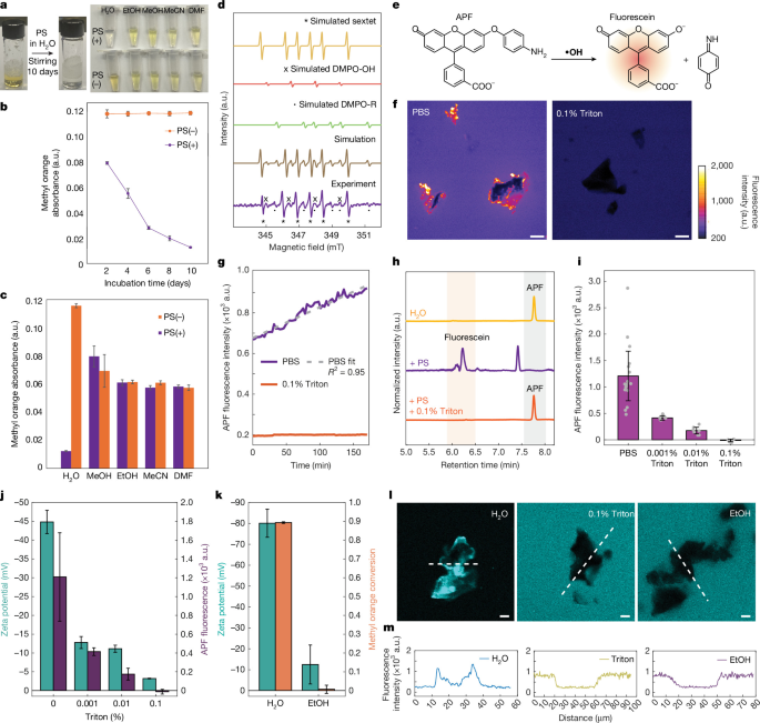
Chemicals and materialsPS microplastic powder with pristine surfaces was purchased with analytical standard grade from Sigma-Aldrich. PS microplastics with different morphologies were purchased from Thermo Fisher and Chem-Impex. The surface purity of model PS microplastics was characterized by X-ray photoelectron spectroscopy (PHI Versaprobe II X-ray Photoelectron Spectroscope) before subsequent experiments. PE, PMMA and PVC were obtained in the format of micrometre-sized powder from Sigma-Aldrich. PET and PP powder were purchased from Goodfellow and Magerials Science, respectively.Rh800 was obtained from Sigma-Aldrich. DMPO was purchased from TCI America. Triton X-100, methyl orange and ThT were obtained from Thermo Fisher. APF (Thermo Fisher Scientific) was obtained as 5 mM stock in N,N-dimethylformamide (DMF) and freshly diluted with phosphate-buffered saline (PBS; pH 7.4) to working concentrations before imaging for robust fluorescence quantification under a microscope. R-PE (BioLegend) and WGA–Alexa Fluor 647 conjugate (Thermo Fisher Scientific) were used as model charged biomolecules to visualize distribution at plastic surface. Alexa 660-labelled single-stranded DNA (5′-Alexa 660-CAC GCG AAG ACT TAA GAT A-3′) was synthesized and purified by Integrated DNA Technologies.All aqueous solutions were prepared using Milli-Q ultrapure water (18.2 MΩ·cm). Solvents including methanol (MeOH), ethanol (EtOH), acetonitrile (MeCN) and DMF were of HPLC grade. Standard buffers and salts (NaCl, FeCl2, NaOH, triethylammonium acetate and trifluoroacetic acid) were purchased from Sigma-Aldrich unless otherwise specified.Microscopy consumables, including glass coverslips, were pre-cleaned by piranha solution (3:1 H2SO4:H2O2) followed by copious rinsing with water unless otherwise specified. Disposable cuvettes were used for zeta-potential measurements with a Malvern ZS Nanosizer instrument.Methyl orange degradationMethyl orange solution (20 µM) was prepared with different solvents (that is, H2O, MeOH, EtOH, MeCN and DMF) and mixed with PS powder (Sigma-Aldrich) at 10 mg ml−1 concentration. The obtained suspension or solution was kept stirring at room temperature at a stir rate of 900 rpm for 10 days. Aliquots were taken every 2 days to monitor the possible degradation of methyl orange. Suspensions were centrifuged at 16,000 rpm for 3 min to obtain the supernatant. Methyl orange absorbance was calculated as OD465nm–OD700nm , where OD465nm and OD700nm are the optical densities measured at 465 and 700 nm, respectively. Subtraction of OD700nm corrected for background signal, including scattering from residual particles. Supernatants were measured in three technical replicate wells (100 µl per well) using a 96-well plate reader. Methyl orange solution prepared with the same solvents at the same concentration without PS addition were kept under the same conditions and monitored at the same time as controls.ESR measurementsDMPO was utilized to trap the radicals for ESR spectroscopy detection. To analyse the spontaneous formation of radical species at the PS–water interface, 200 mg PS powder was mixed with 20 mM DMPO solution in water. The suspension was incubated at room temperature for 20 min before filtration to collect the filtrate. The resulting filtrate was transferred into a Wilmad Glass quartz flat cell for ESR spectroscopy measurements. The spectra were acquired at room temperature with a Bruker ELEXSYS E500 EPR spectrometer under the following conditions: microwave power 20.23 mW; 12 scans averaged; centre field 3,480 G; sweep width 100 G; modulation amplitude 1 G; microwave frequency 9.768037 GHz.APF radical sensing assayConfocal fluorescence imagingAPF (5 mM; Thermo Fisher) was diluted to 5 µM using PBS. Then 1 ml of 5 µM APF was mixed with approximately 1 mg of microplastic particles (PP, PS, PE, PET, PVC or PMMA) through vertexing. Aliquots of the mixture were sandwiched in a glass chamber made by an imaging spacer separating the piranha-solution-treated cover glass and glass slide. Confocal fluorescence imaging was performed immediately after sample preparation. The green fluorescence channel was excited with an argon laser at 488 nm and emission was collected within a 505–520 nm band. Time-lapse images were acquired every 3 min with the excitation power optimized to minimize photobleaching and other perturbations during in situ tracking of the fluorogenic APF signal.For endpoint quantification of the APF assay, mixtures containing 5 µM APF and approximately 1 mg of microplastic particles (PP, PS, PE, PET, PVC or PMMA) were first dispersed by vortexing and then incubated in the dark at room temperature for 90 min to allow the fluorogenic reaction to progress at the plastic–water interface. After incubation, aliquots of each sample were mounted in imaging chambers composed of a poly-l-lysine coated coverslip (Neuvitro) and a glass slide separated by a spacer. Fluorescence images were acquired with constant laser power, photomultiplier tube (PMT) voltage, detector gain and pinhole size across all measurements to ensure quantitative comparability. Multiple non-overlapping fields of view were imaged for each polymer type to account for potential spatial heterogeneity in fluorescence signal distribution.Quantification of APF fluorescence was performed after generating maximum-intensity Z projections from the acquired confocal stacks. Particle regions of interest were segmented using corresponding stimulated Raman scattering (SRS) images as references to accurately define particle boundaries. The fluorescence intensities were then extracted as area-weighted averages from the segmented regions of interest to represent the relative reactivity of each microplastic type.SRS imagingWe used SRS imaging to characterize microplastics together with confocal imaging analysis54. SRS imaging was conducted on a confocal laser-scanning microscope (FV1200, Olympus) integrated with customized laser sources. A commercial laser system (PicoEmerald S, Applied Physics & Electronics) provided both the pump and Stokes beams. The Stokes wavelenghth was fixed at 1,031.8 nm and modulated at 20 MHz by an electro-optic modulator, whereas the pump beam was tunable and set to 784.2 nm to excite C–H vibrational modes characteristic of microplastics. Both beams with an approximately 2-ps pulse width and 80-MHz repetition rate, were spatially and temporally synchronized, and tightly focused onto the sample using a ×25 water-immersion objective (XLPlan N, 1.05 NA MP, Olympus). The transmitted beams were collected by an oil-immersion condenser with a numerical aperture of 1.4, with the Stokes beam removed by a high-optical-density bandpass filter (890/220 CARS, Chroma Technology). The transmitted pump beam was detected by a silicon photodiode (S3590-09, Hamamatsu) under 64-V bias. The photodiode output was terminated through a 50-Ω load, and demodulated using a high-frequency lock-in amplifier (HF2LI, Zurich Instruments) at 20 MHz. The demodulated pump-loss signal was digitized and transmitted to the FV10 analogue input channel to generate SRS images.HPLC analysisAn Agilent 1200 series system equipped with a Vydac 218TP-C18 column (250 × 4.6 mm, 5 µm; Grace) was utilized for HPLC analysis. The gradient was increased from 5% B to 95% B in 15 min (solvent A, water + 0.1 M triethylammonium acetate; solvent B, acetonitrile + 0.1% (v/v) trifluoroacetic acid). The detection unit was set to monitor the reaction by the absorbance at 488 nm. The peaks corresponding to APF and its oxidation product, fluorescein, were assigned based on the retention time measured from the standard solution.To examine the APF conversion in water upon PS powder addition, 100 mg PS powder was suspended in 1 ml of 20 µM APF solution in water with and without 0.1% Triton X-100 supplement. The suspension was left stirring in the dark for 16 h at room temperature before filtration to collect the filtrate for HPLC analysis. A positive control was prepared by mixing 20 µM APF with 20 mM H2O2 and 2 mM FeCl2 in water and incubated for the same duration before HPLC analysis.Surface localization imaging assaySurface localization of charged fluorophorePS particles (1 mg ml−1) were suspended in 1 µM Rh800 prepared under different solvent conditions (that is, H2O, 0.1% Triton X-100 in H2O, and EtOH). The suspensions were incubated in the dark at room temperature for 10 min before confocal fluorescence imaging. The far-red channel was excited by an 635-nm laser with a collection band of 655–755 nm.Surface localization of proteinPlastic particles (10 mg ml−1) were mixed with protein in PBS (0.02 mg ml−1) to image the surface of absorption of the protein under confocal fluorescence imaging. Proteins with different net charges in the PBS environment were selected with R-PE (Biolegend) being negatively charged and WGA (Thermo Fisher, W32466) being positively charged at pH 7.4. The mixture was vortexed and incubated in the dark for 15 min before an aliquot of the mixture was sandwiched in a glass chamber in the same way with piranha-solution-treated cover glass. WGA conjugated with Alexa Fluor 647 was imaged in the far-red channel, excited by an 635-nm laser with fluorescence collected between 655 nm and 755 nm. R-PE was imaged in the red channel, excited by a HeNe(G) laser (543 nm) with emission collected between 560 nm and 660 nm. Simultaneous imaging of the two channels revealed the different partition pattern of oppositely charged proteins on plastic surfaces.Surface localization of DNAAlexa 660-labelled DNA (500 nM; 5′-Alexa 660-CAC GCG AAG ACT TAA GAT A-3′, from Integrated DNA Technologies) was added to plastic particles (approximately 10 mg ml−1) to image the surface adsorption of the DNA molecules under confocal fluorescence imaging. The mixture was vortexed and incubated in the dark for 15 min before an aliquot of the mixture was sandwiched in a glass chamber in the same way with a piranha-solution-treated cover glass for confocal imaging with the far-red channel excited by an 635-nm laser, and emission was collected at 655–755 nm.ThT assay for protein aggregation analysisThT is widely used as a ‘gold standard’ for selectively staining and identifying amyloid fibril formation both in vivo and in vitro55. Here, 0.1 mg ml−1 lysozyme solution stained with 20 μM ThT in PBS was mixed with plastic particles at a concentration of 1 mg ml−1. The mixture was vortexed before an aliquot was sandwiched in a glass chamber in the same way with a piranha-solution-treated cover glass for confocal fluorescence imaging. ThT fluorescence was excited at 488 nm and collected in the 505–520 nm emission window. Time-lapse imaging was performed on selected particles at 5-min intervals.Fluorescence images for quantification of the ThT assay for different microplastics were acquired after incubating the mixture in the dark for 2 h. z-stack images were acquired for each region of interest to map the thioflavin fluorescence at the particle surface. Quantification of the fluorescence signal are performed after z-stack projection (maximum intensity) by segmenting the particles in reference to the corresponding SRS images (method described in ‘SRS imaging’) and measured the area-weighted average fluorescence for segmented particle regions of interest.For the experiment comparing the effect of radical scavenger on protein aggregation at the PS–water interface, ThT fluorescence was monitored using a BioTek Cytation 9 Cell Imaging Multimode Reader. Samples containing 4 mg ml−1 PS microplastics, 0.1 mg ml−1 lysozyme and 20 μM ThT in PBS, with or without 100 mM caffeine, were prepared in a 24-well plate and imaged as z-stacks with a ×20 objective before and after a 4-h incubation at 37 °C in the dark inside the instrument. A 4% agarose gel pad prepared in PBS to minimize particle movement in solution during imaging. Five to six fields of view were defined for each condition and the same particle retained within each field at the two time points were identified and analysed. Surface-associated ThT fluorescence was quantified as the average fluorescence intensity over the particle area, and the fluorescence change for each particle was calculated as Ft/F0, where F0 and Ft denote the surface fluorescence of the same particle before and after incubation, respectively.Haemolytic assayMouse whole blood was collected from wild-type mice (BALB/cJ, 20 weeks old, Jackson Lab) with an animal protocol (AC-AABN0554) approved by the Institutional Animal Care and Use Committee (IACUC) at Columbia University. A final concentration of approximate 10 mM EDTA was supplemented to prevent coagulation. Haemolysis was assessed using a published protocol56. As soon as possible after phlebotomy, the blood samples were centrifuged at 1,700 g for 5 min. The supernatant was removed by aspiration and 2 ml PBS pH 7 was added. The washing step was repeated three times or until the supernatant was clear. After final aspiration, the remaining pellet was diluted in PBS (1:100) to obtain erythrocyte suspension. To test haemolytic activity, 150 μl of obtained erythrocyte suspension was gently mixed with 2 mg plastic particles and incubated for 60 min at 37 °C without agitation before centrifuged at 1,700g for 5 min to collect the supernatant. The same erythrocyte suspension with no plastic particles was examined as a negative control. Haemolytic activity was then quantified by measuring optical density at 405 nm (OD405nm) of the supernatant using a plate reader with 96-well plates.Zeta-potential measurementThe electrophoretic mobilities of PS particles in different conditions were measured using a Malvern ZS Nanosizer instrument. Pristine PS microparticles or carboxylic-acid-functionalized PS microparticles were prepared with a concentration of 1 mg ml−1 in 1 mM NaCl aqueous solution to examine the sensitivity of their surface electrostatics to different concentrations of Triton X-100 supplement. Pure water and ethanol were also used to suspend the pristine PS microparticles or carboxylic-acid-functionalized PS microparticles at the same concentration to compare their solvent sensitivity to the surface electrostatics. Zeta-potential (ζ) values were calculated from the electrophoretic mobility values using the following expression: \(\mu =\frac{\varepsilon {\varepsilon }_{0}}{\eta }\zeta f(\kappa a)\), where ε0 is the vacuum permittivity, ε is the relative permittivity of solvent, η is the viscosity of solvent and f(κa) is Henry’s function. The Hückel formula was used to calculate the zeta potential and compare between different samples15. All measurements were performed at 25 °C with disposable plastic cuvettes.Theory and simulationNon-reactive and reactive force fieldsFor many of the structural analyses used in this study, we used the force-field combination of OPLS-AA for the polymer and the SPC/E water model. However, to generate configurations for the VIE calculations, we used a more sophisticated ReaxFF/C-GeM model to describe water, OH− and Na+. Previous studies have shown that classical fixed-charge OH− force fields often predict overcoordinated hydration environments, frequently yielding coordination numbers exceeding six. In contrast, ab initio simulations and experimental evidence indicate that hydroxide is best described as a hypercoordinated species with approximately three to five hydrogen bonds. In this context, reactive force-field approaches such as ReaxFF/C-GeM provide a more physical description by explicitly accounting for charge redistribution and proton-transfer dynamics. ReaxFF/C-GeM has been shown to accurately capture the energetics and dynamics of hydronium and hydroxide ion species57. In particular, proton-transfer events that interconvert different hydration states of hydroxide (for example, transitions between four- and three-hydrogen-bond configurations) have been identified as rate-controlling steps for hydroxide diffusion. ReaxFF/C-GeM has been shown to reproduce both the solvated structure of hydroxide and its diffusion coefficient in water with reasonable accuracy (for example, approximately 0.40 Å2 ps−1 from ReaxFF/C-GeM compared with approximately 0.56 Å2 ps−1 experimentally). Such capabilities are especially relevant for resolving interfacial hydration structure and ion mobility at polymer–water interfaces, which are central to the present study.Electrostatic embedding model for ReaxFF/C-GeMIn this study, we performed MD simulations of an interfacial system of an aqueous NaOH solution with three microplastic systems in a slab geometry using an electrostatic embedding scheme by modelling the water and NaOH with the reactive force-field ReaxFF/C-GeM57,58, and used the non-reactive OPLS-AA59,60 for PE, PVC and PMMA. The system is partitioned into three components:
1.
ReaxFF/C-GeM atoms, which include all water and NaOH and are treated using the reactive force field.
2.
All polymer atoms are described entirely by a non-reactive (OPLS-AA) force field.
3.
Non-bonded interactions between the ReaxFF/C-GeM and OPLS-AA regions, including van der Waals and electrostatic interactions, which provide the coupling between the two force-field descriptions. For the van der Waals interactions, we adopt parameters consistent with the OPLS-AA/SPC/E force field, following the same protocol established in our previous work on reverse micelle systems61 and using the standard mixing rules of the OPLS force field. Water–polymer electrostatics are treated with fixed charges for the polymer and Gaussian charge density for the water and NaOH. See refs. 61,62 for further details.
Importantly, this electrostatic embedding modelling strategy has been used and validated in previous studies, including systems involving both neutral and charged reverse micelles61,62. In those studies, the force-field combination was benchmarked against a range of experimental observables from dielectric relaxation and terahertz spectroscopy related to interfacial proton-transfer-related phenomena61,62.Further benchmarking of force-field combinationsWe have also evaluated interaction energies and hydrogen-bond-related intermolecular distances for representative polymer–water model systems (Supplementary Table 1), constructed from small-molecule analogues and optimized consistently at each level of theory. As shown in Supplementary Table 1, both OPLS-AA/SPC/E and OPLS-AA/ReaxFF-C-GeM reproduce the correct qualitative trends in interaction strength across the different systems. Notably, the OPLS-AA/ReaxFF-C-GeM model shows improved agreement with density functional theory in both binding energies and intermolecular distances, particularly for PMMA, where stronger hydrogen-bonding interactions are more accurately captured. These results support that the hybrid OPLS-AA/ReaxFF-C-GeM approach provides a physically reasonable and reliable description of polymer–water interactions at the interface.In addition, radial distribution functions between water and representative polymer surface atoms further confirm that both force-field descriptions yield consistent interfacial hydration structures, with only minor quantitative differences, as seen in Extended Data Fig. 7a–f. The two force-field descriptions (OPLS-AA/SPC/E and OPLS-AA/ReaxFF-C-GeM) yield overall consistent radial distribution function profiles across the three systems. For the PMMA system, the OPLS-AA/ReaxFF-C-GeM model exhibits a more pronounced first peak, indicating stronger water–polymer interactions. This is consistent with interaction energy analysis, which shows that hydrogen-bonding interactions are stronger in the OPLS-AA/ReaxFF-C-GeM description compared with OPLS-AA/SPC/E. Notably, this stronger interaction is in closer agreement with density-functional-theory-level calculations, suggesting that the ReaxFF/C-GeM-based description provides a more accurate representation of interfacial hydrogen bonding in this system.Simulation details for OPLS-AA/SPC/E used for structural analysisFor water–plastic interfaces, plastics and Triton X-100 surfactant molecules were modelled with the all-atom OPLS-AA force field59,60 and water using the SPC/E model. Each system consisted of a single long polymer chain in a slab geometry of approximately 40,000 polymer atoms and approximately 9,000 water molecules. Non-bonded interactions were truncated at 10 Å, and for SPC/E long-range electrostatics were computed using the particle–particle particle-mesh Ewald method with a convergence criterion of 10−5. The molecular dynamics simulations were carried out using LAMMPS63, and used a 1-fs timestep with SHAKE constraints applied to SPC/E water molecules64. The temperature was maintained at 300 K using a Nosé–Hoover thermostat (damping constant 100 fs)65, and constant pressure in the z direction (1 atm) was enforced.The initial polymer slabs were prepared following the protocol previously described44. The polymer systems were first equilibrated for 500 ps before introducing SPC/E water. After adding water above the slab, the system was further relaxed and equilibrated for 1 ns, followed by a 5-ns production run. Snapshots were saved every 10 ps, yielding 500 frames for structural analysis presented in Fig. 3d,e, and in Extended Data Figs. 4–6 and 7a–f.Simulation details for OPLS-AA/ReaxFF-C-GeM used for structural analysisWe performed molecular dynamic simulations with the electrostatic embedded model using a modified version of LAMMPS for PE, PVC and PMMA58. Each system consisted of a single long polymer chain in a slab geometry of approximately 8,000 polymer atoms and approximately 2,000 water molecules for ReaxFF/C-GeM. Non-bonded interactions were truncated at 10 Å. The simulations used a 0.25-fs timestep, the temperature was maintained at 300 K using a Nosé–Hoover thermostat (damping constant 100 fs)65 and a constant pressure in the z direction (1 atm) was enforced. The initial polymer slabs were prepared following the protocol previously described44. The polymer systems were first equilibrated for 500 ps before introducing water. After adding water above the slab, the system was further relaxed and equilibrated for 400 ps using ReaxFF/C-GeM, followed by a 2-ns production run. Snapshots were saved every 5 ps, yielding 400 frames for ReaxFF/C-GeM for structural analysis in Fig. 3e and in Extended Data Figs. 7 and 8.Simulation quantities for the microplasticsTo better characterize the polymer surfaces in our OPLS-AA simulations, we analysed both the polymer density and the distribution of exposed functional groups at the interface. Supplementary Table 2 shows that the equilibrated microplastic systems reproduce physically reasonable bulk densities using a standard 21-step protocol66. We also computed the surface-exposed functional groups density profile, ρpoly(z), to identify the interfacial region. Within this region, surface-exposed functional groups were defined as those located within 4 Å of the Willard–Chandler interface (WCI, the instantaneous interface defined as the isodensity surface of the water oxygen density field at half of the bulk liquid density). We then evaluated the surface density of functional groups for each polymer system. As PE does not contain functional groups, it is not included in this analysis. For the other systems, we selected representative groups: chlorine atoms for PVC, the two oxygen atoms in the COOR group for PET and PMMA, and the aromatic ring centroid for PS. As shown in Extended Data Fig. 8a, the surface functional group densities exhibit narrow distributions, with relative fluctuations below approximately 5%, indicating that the exposed surface composition remains stable over the course of the simulation, without significant interfacial reconstruction. Furthermore, comparisons between OPLS-AA/SPC/E and OPLS-AA/ReaxFF-C-GeM show only minor differences in the distributions, suggesting that the interfacial functional group exposure is robust with respect to the choice of water model. These results indicate that, although the polymer matrices are amorphous, the interfacial surface structure remains statistically stable on the simulation timescale, supporting the reliability of the observed hydration and reactivity trends. Together, these results support the use of a single-chain representation for the present interfacial study.VIE calculations and sampling detailsFor VIE calculations, 4 NaOH molecules were added to the water phase (box size approximately 3.6 × 3.6 × 7 nm3) based on the surface charge density reported in ref. 42. VIEs were computed following the procedure in ref. 19 at the ωB97M-V level of theory using Q-Chem67, with aug-cc-pVTZ for OH−/OH• and aug-cc-pVDZ for surrounding environments. Each calculation included explicit solvent within 6 Å of the hydroxide ion, with the remainder treated via charge embedding from atomic charges from the remaining simulated environment. Hydrogen bonds to OH− were defined by a donor(water-H)–acceptor(O–H−) distance ≤2.7 Å and an O–H–O angle ≥115°. All results are shown in Fig. 3a.As the experimentally measured zeta potential reflects the potential at the slip plane, this implies a net charge imbalance within the interfacial region, that is, the particle effectively carries excess negative charge. To model this, we removed all Na+ ion as a practical way to reproduce this charge imbalance in a finite simulation set-up. Explicitly resolving the electrical double layer would require substantially larger system sizes and longer timescales than are currently feasible. Removing Na+ therefore provides a simple but direct way to impose an experimentally motivated interfacial charge density consistent with experimentally measured zeta potentials. All results are shown in Fig. 3c.In our VIE calculations, configurations are constructed by including explicit solvent molecules within 6 Å of the hydroxide ion, which may exclude direct polymer–OH− contacts in some interfacial configurations. To assess the impact of this approximation, we directly compared VIE values computed with and without configurations involving the OH− proximity to the PE plastic. As shown in Extended Data Fig. 7g, the two sets of results are in close agreement on a per-configuration basis, with data points distributed near the parity line. The average VIE values are 192.99 kcal mol−1 and 193.82 kcal mol−1, differing by only 0.83 kcal mol−1 (To ensure consistency and convergence across systems, all molecular dynamics simulations using ReaxFF/C-GeM are over a timescale of 2 ns for each polymer–water system. The time-resolved VIE distributions show that the statistics are well converged over the simulation timescale, whereas the spatial distributions of undercoordinated hydroxide ions relative to the interface are consistent with the observed trends in VIE behaviour across different polymer systems. The results shown in the main text (Fig. 3a,c) were obtained from one representative 500-ps trajectory window, from which configurations were sampled every 2.5 ps. By contrast, Extended Data Fig. 8c–e is included primarily to demonstrate convergence across the full 2-ns simulation. For this analysis, the trajectory was divided into 4 consecutive 500-ps windows, and configurations were sampled every 5 ps within each window, yielding approximately 100 configurations per segment. Owing to occasional SCF convergence failures in the electronic-structure calculations, the number of successfully evaluated configurations is slightly reduced but remains sufficient to construct statistically meaningful VIE distributions. To improve the sampling of rare interfacial configurations, we additionally used a targeted sampling scheme based on structural criteria (distance to the WCI 8c–e, the time-resolved VIE distributions reveal distinct behaviours across the three polymer systems. In the PE system, a low-VIE tail is observed in both the early and late trajectory segments, indicating that such configurations are sampled repeatedly over the course of the simulation. In the PVC system, a low-VIE tail emerges in the later trajectory segment (1.5–2.0 ns), consistent with the behaviour observed in PE, but with lower frequency, reflecting the presence of rare interfacial configurations. In contrast, as shown in Extended Data Fig. 8b, the PMMA system exhibits a substantially lower population of undercoordinated hydroxide ions in the interfacial region, and no configurations corresponding to the low-VIE tail are observed over the full 2-ns simulation. These observations further support the connection between interfacial hydroxide structure and VIE behaviour across different polymer systems.