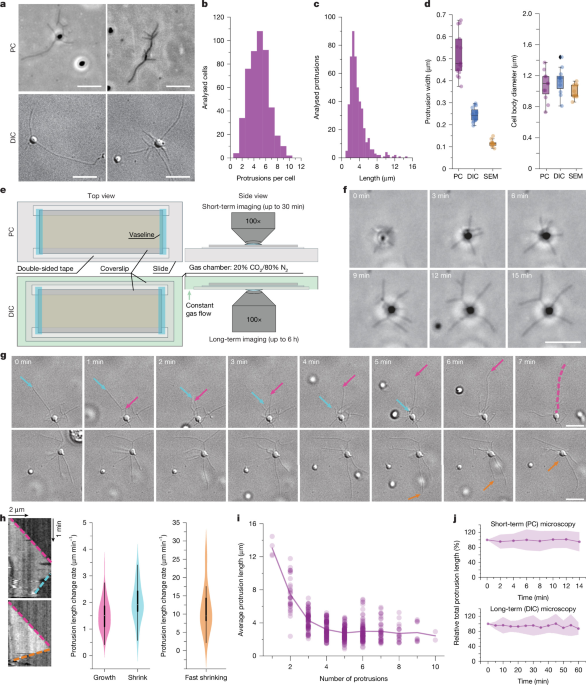
Cultivation of Ca. L. ossiferum and M. peptidophilumCa. L. ossiferum enrichment cultures were grown protected from light in lokiarchaeal media in sealed, pressurized serum bottles in an 80:20% N2:CO2 atmosphere (0.3 bars) at 20 °C without shaking, as described previously7. The growth medium composition (per litre) was as follows: 20.7 g NaCl, 5 g MgCl2·6H2O, 2.7 g NaHCO3, 1.36 g CaCl2·2H2O, 0.54 g NH4Cl, 0.14 g KH2PO4, 0.03 g Na2S·9H2O, 0.03 g cysteine·HCl, 0.5 ml of acid trace element solution, 0.5 ml of alkaline trace element solution, 1 ml Se/W solution, 0.1% casein hydrolysate (w/v). The acid trace element solution contained (per litre): 1.49 g FeCl2·4H2O, 0.062 g H3BO3, 0.068 g ZnCl2, 0.017 g CuCl2·H2O, 0.099 g MnCl2·4H2O, 0.119 g CoCl2·6H2O, 0.024 g NiCl2·6H2O and 4.106 ml of 37% HCl. The alkaline trace element solution contained (per litre): 0.017 g Na2SeO3, 0.033 g Na2WO4, 0.021 g Na2MoO4 and 0.4 g NaOH. The pH was adjusted to 7.5, and the medium was supplemented with ampicillin, kanamycin and streptomycin (200 μg ml−1 each). The cultures were continuously passaged into serum flasks containing fresh medium—typically using an early stationary-phase culture as inoculum (1:10 dilution). Growth of L. ossiferum cultures was monitored by qPCR using lokiarchaeal-specific primers for 16S rRNA as described previously7. Ca. M. peptidophilum HC1 was grown in casamino acids–peptone–yeast extract medium in sealed serum bottles in an N2 atmosphere at 30 °C as described9. qPCR results were used to select cultures for live-cell imaging, and only cultures with densities above 1 × 10⁶ L. ossiferum per ml and a relative abundance of L. ossiferum above 20% were chosen. Cultures were in late exponential or stationary phase and between 15 days and 40 days old. Live imaging of M. peptidophilum was performed on cultures in the late exponential to early stationary phases with a population ratio of HC1:MC2 = 70:30%.Immunofluorescence and microscopy of fixed cellsFor immunofluorescence experiments, L. ossiferum cultures were transferred onto poly-l-lysine (0.01%)-coated coverslips and incubated for 45 min in anaerobic conditions. Cells were then fixed with 3.7% PFA in PEM buffer (80 mM PIPES, 2 mM MgCl2 and 0.5 mM EGTA at pH 6.9). The cells were permeabilized with 0.1% Triton X-100 and blocked with 1% BSA solution in PBS-T. The primary antibody against Lokiactin and the secondary antibody (goat anti-rabbit AlexaFluor488, abcam ab150077) + 1 mg ml−1 Hoechst were diluted 1:1,000 in PBS-T + 0.1% BSA and either incubated for 1 h (primary) or 0.5 h (secondary) at room temperature, protected from light. Meanwhile, coverslips were washed gently with PBS by changing the solution twice. Finally, the coverslips were mounted using the VECTASHIELD antifading agent. The Lokiactin antibody was raised against a Lokiactin-specific peptide (CTFYTDLRVDPSEHPV) and previously validated by ELISA, western blot and immunogold localization7. To compare DNA signals and morphologies of L. ossiferum and their symbionts, cultures were fixed with 0.5% glutaraldehyde for 20 min, and DNA was simultaneously stained with Hoechst 33342 (1:1,000 dilution of 1 mg ml−1 stock solution). After fixation, cells were centrifuged 2× for 10 min at 15,000g, and the resulting pellet was resuspended in Milli-Q to remove traces of glutaraldehyde and media. The cell suspension was dried 6 min at 65 °C and subsequently mounted using VectaShield antifading agent. Fixed cells were imaged with a Nikon Eclipse upright microscope equipped with a 100× Nikon 1.45 PlanApo oil objective.Preparation of flow chambers and live imagingFor upright phase contrast imaging, flow chambers were prepared with a Soda Lime microscopy slide (1 × 24 × 75 mm, bottom) and a Soda Lime coverslip (0.17 × 24 × 40 mm, top, Fisher Scientific 11348503). Two strips of double-sided sticky tape were placed on the outer edges of the bottom glass and sealed. After assembly, flow chambers were incubated in a 20:80% N2:CO2 atmosphere for at least 2 h. A total of 100 µl of a Loki culture was sampled and transferred into a 2 ml Eppendorf tube filled with 20:80% N2:CO2. Subsequently, 50 µl of the culture were loaded into the flow chamber within an anoxic atmosphere. The flow chambers were sealed with Vaseline to avoid oxygen exposure in the phase contrast setup. The cells were incubated for at least 90 min before starting imaging experiments in a 20:80% N2:CO2 atmosphere. Time-lapse experiments were performed with an upright Nikon Eclipse microscope, equipped with a 100× Nikon 1.45 PlanApo oil objective and a phase contrast setup. Videos were acquired with a frame rate of 2 s and for a maximum of 30 min before placing the slide again into an anoxic chamber. For poly-l-lysine experiments, the bottom slide was coated with different concentrations of poly-l-lysine for 10 min, washed extensively with Milli-Q H2O and dried for 2 h at 60 °C. Flow chambers were assembled and imaged as described above. For inverted DIC microscopy, flow chambers were prepared as described above, but the bottom glass was exchanged with a thinner Soda Lime coverslip (0.17 × 24 × 50 mm, Fisher Scientific 12303148). DIC experiments were performed with a Nikon Ti2-E microscope, equipped with a 100× Nikon 1.45 PlanApo oil objective. The imaging slide was mounted with a custom-printed 3D slide holder and a custom slide holder stage. Next, a gas chamber was placed on top, enabling environmental control of the atmosphere surrounding the slide. The temperature was kept at 22 °C, and the atmosphere of the gas chamber was kept at 15:85% N2:CO2 by flowing in the gases at a flow rate of 13 l h−1 using an ibidi gas mixer. Oxygen levels were checked with Anaerostrips placed next to the flow chamber. The sealing with Vaseline minimized evaporation of the liquid over the course of the imaging experiment. DIC experiments were recorded with frame rates of 5–60 s, depending on the number of positions imaged and for a maximum of 6 h.For live imaging experiments with fluorescently labelled DNA, 1 drop of NucBlue was added to 1 ml of culture before loading the flow chamber. Images were recorded every 60 s, with 20 ms exposure time and 1% power of the 405 nm Lumencor LED light source. For live fluorescence imaging of Lokiactin, we diluted the FastAct stock solution 1:1,000 directly with the L. ossiferum culture before loading the flow chamber, followed by incubation for at least 3 h. Images were recorded every 10–30 s, using a 50 ms exposure time and 25% power of the 640 nm Lumencor LED light source. Conditions for the experiments with SiR-Actin and FastAct_X were the same, and likewise for experiments with FastAct and Swin A except for the additional incubation with 250 ng ml−1 Swin A.Actin inhibitor experimentsInitial experiments of actin inhibitors were performed at 25 µg ml−1, 12.5 µg ml−1 or 5 µg ml−1 final concentrations (Supplementary Table 1). For these experiments, we used a single culture (24 days, 1.73 × 10⁷ L. ossiferum per ml and 58% relative abundance) and tested the effect of seven inhibitors each on three subsequent days, to ensure that inhibitor effects are not affected by changes in the cell cycle. We used concentrations higher than what is recommended for eukaryotic cells to compensate for potentially lower, hampered affinities for Lokiactin. Subsequent titration experiments were performed with inhibitors that had affected the morphology and protrusions of L. ossiferum in the initial screen. For this, we performed a serial dilution of the inhibitors (stock solutions either 1 mg ml−1 or 2.5 mg ml−1) in DMSO to reach concentrations from 250 to 0.25 µg ml−1 or 100 to 0.1 µg ml−1. We then added 1 µl from each inhibitor dilution to 199 µl of L. ossiferum culture in an N2:CO2 atmosphere. These titrations were performed with a single culture (25–28 days, 4.21 × 10⁶ L. ossiferum per ml, 22.57% relative abundance) for Chaetoglobosin A and Pseudofuscochalasin A. For Aspochalasin D and Swin A, titrations were performed with two L. ossiferum cultures (27 days old and 35 days old, 3.1 × 10⁶ and 4.3 × 10⁶ L. ossiferum per ml, 20% and 22% relative abundance). More details about the used actin inhibitors are provided in Supplementary Table 1.Image analysisImage analysis in this study was performed with FIJI61. All plots have been created with Jupyter Notebook and all box plots indicate the median using the central line within the box, and the lower and upper boundaries of the box represent the first (Q1) and third (Q3) quartiles, respectively. Whiskers extend to the most extreme data points within 1.5 × interquartile range of Q1 and Q3. Individual points beyond the whiskers are shown as outliers. For colour coding the protrusion growth shown in Extended Data Fig. 1h, the time-lapse was first stabilized targeting the cell body, smoothed with a walking average of four frames and then subsampled every 30th frame. The resulting video was colour-coded using the Temporal-Color Code plugin and the mpl-magma lookup table. To measure the rates of protrusion growth and shrinking, regions of interest with single L. ossiferum cells were selected from videos and stabilized using the cell body as a matching template. Then, a line was drawn along the protrusion of interest, and a kymograph was created using the reslice command. The rate was determined by measuring the distance travelled over time.Measuring protrusion dimensions and the change of lengthTo measure the length of protrusions over time, single cells were selected, and the total length of all protrusions measured with the segmented line tool every 1 min or 5 min for a total of 15 min (phase contrast) or 60 min (differential interference contrast). The change in length (∆L) was calculated by \(\Delta L=\frac{{L}_{0}}{{L}_{{i}}}\ast 100\), where L0 is the total length of the first time point and Li the total length in subsequent frames. The diameter of protrusions and the cell body of cells was determined by extracting intensity line profiles from a line with line width = 5 and extracting the full width at half maximum from a Gaussian fit to the line profiles of either protrusions or cell bodies.Tracking cell migrationTo quantify cell migration, we selected mobile cells and analysed the regions of interest. Videos were inverted, their contrast normalized for analysis, and cell bodies tracked with TrackMate62. Trajectories were built using the LAP tracker, allowing a linking maximum distance of 1 µm, a gap-closing max distance of 2 µm and a frame gap of a maximum of five frames. The resulting trajectories were manually curated, to avoid faulty linking due to focus shifts or floating of other, unbound cells into the field of view. Velocities, confinement ratio, track durations and displacements were recovered from corresponding .csv and .xml files. To determine the impact of protrusions on the migration direction, cells were manually segmented and used to train a pixel classification model in ilastik for automated detection of cell bodies and protrusion tips. Cell body trajectories were extracted with the TrackMate plug-in in Fiji. The movement direction was defined by the displacement vector between consecutive cell body centroids. For each frame, protrusion vectors were drawn from the cell centroid to each tip, and their alignment with the movement vector was calculated as the cosine of the included angle. Two metrics were derived: (1) the mean alignment, corresponding to the average cosine across all protrusions, and (2) the weighted alignment, given by the sum of cosines weighted by protrusion lengths (tip to centroid distances) and normalized by total protrusion length. Both indices range from −1 (protrusions opposing movement) to +1 (protrusions aligned with movement).Quantifying the effect of actin inhibitors on L. ossiferumTo assess the initial effect of inhibitors, we quantified the number of L. ossiferum cells with protrusions adhered to the glass slide after 90 min of incubation. For an in-depth analysis, the number of protrusions of each L. ossiferum cell in the presence of different concentrations of Swin A was counted, and we measured protrusion change length rates by kymography, as described above. To quantify the intensity of FastAct in the absence and presence of Swin A, we extracted line intensity profiles of the FastAct channel along the cell body or the protrusion with ImageJ. For each line profile, we estimated background fluorescence from the first five data points and subtracted it them from the entire profile, setting negative values to zero. The background-corrected signal was then integrated along the cell axis using trapezoidal integration. To account for differences in cell length, the integrated intensity was normalized by the profile length, yielding the mean fluorescence intensity per μm.Culture preparation for Co-IP experimentsFor Co-IP, we selected three large-scale cultures (500 ml each) in stationary phase (1 × 47 days and 2 × 40 days old) at densities of 1.8–3.5 × 10⁶ L. ossiferum per ml and relative abundances above 20%. For fixation, formaldehyde was added to the cultures at a final concentration of 0.25% and incubated for 20 min with gentle agitation. Crosslinking was quenched by adding glycine to a final concentration of 250 mM for 5 min, followed by centrifugation and two washes with base medium. For immunoprecipitation, 10 µg of antibody was coupled using the Pierce Crosslink Magnetic IP/Co-IP Kit (Thermo Fisher), including crosslinking with DSS according to the manufacturer’s protocol. Cells were lysed in lysis buffer containing 50 mM Tris-HCl (pH 7.4), 150 mM NaCl, 10 mM MgCl2, 1 mM EDTA, 0.1% IGEPAL CA-630, and a protease inhibitor tablet. Lysates were sonicated (1 s on and 3 s off, 20% amplitude, 2 min) and centrifuged. Protein concentration was measured and 200 µg of protein from the supernatant of each culture incubated overnight with Lokiactin-antibody-coupled beads and IgG-coupled beads (Abcam) as a negative control. Beads were washed twice with a detergent-free buffer (20 mM Tris-HCl pH 7.5, 75 mM NaCl).Sample preparation for mass spectrometry analysis of Co-IP experimentsThe beads were resuspended in 30 µl 2 M urea and 50 mM ammonium bicarbonate. The beads were digested with 150 ng LysC (mass spectrometry grade, FUJIFILM Wako chemicals) at room temperature for 90 min. The supernatant was transferred to a new tube. The beads were rinsed with 30 µl 50 mM ammonium bicarbonate and combined with the supernatant. Disulfide bonds were reduced with 2.4 µl of 250 mM dithiothreitol (DTT) for 30 min at room temperature before adding 2.4 µl of 500 mM iodoacetamide and incubating for 30 min at room temperature in the dark. The remaining iodoacetamide was quenched with 1.2 µl of 250 mM DTT for 10 min. Proteins were digested with 150 ng trypsin (Trypsin Gold, Promega) in 1.5 µl 50 mM ammonium bicarbonate overnight. The digest was stopped by adding trifluoroacetic acid (TFA) to a final concentration of 0.5%, and the peptides were desalted using C18 Stagetips63.Liquid chromatography-mass spectrometry analysis of Co-IP experimentsLiquid chromatography-mass spectrometry analysis was performed on a Vanquish Neo UHPLC system (Thermo Scientific) coupled to a timsTOF HT (Bruker). The system was equipped with a CaptiveSpray ion source (Bruker) and a column oven (Sonation). Peptides were loaded onto a trap column (PepMap Neo C18 5 mm × 300 µm, 5 μm particle size, Thermo Scientific) using 0.1% TFA as mobile phase, and separated on an analytical column Aurora Ultimate XT C18, 25 cm × 75 µm, 1.7 µm particle size, IonOpticks, applying a linear gradient starting with a mobile phase of 98% solvent A (0.1% FA) and 2% solvent B (80% acetonitrile, 0.08% FA), increasing to 35% solvent B over 60 min at a flow rate of 300 nl min−1. The analytical column was heated to 50 °C. The mass spectrometer was operated in data-dependent acquisition (DDA) parallel accumulation serial fragmentation (PASEF) mode. MS2 data were acquired with 10 PASEF scans per duty cycle. The ion mobility range was set to 0.64–1.42 V s cm−1, and the accumulation and ramp time was set to 100 m. Precursor ions were selected for fragmentation using an isolation window of 2m/z for m/z m/z for m/z > 700. The precursor intensity threshold was set to 2,500, precursor repetitions were enabled with a target intensity of 20,000, and active exclusion was enabled with a 0.4 min release delay. Singly charged precursor ions were excluded using a polygonal filter applied in m/z-ion mobility space. TIMS elution voltages were calibrated linearly to obtain the reduced ion mobility coefficients (1/K0) using three Agilent ESI-L Tuning Mix ions (m/z 622, 922 and 1,222). Collision energy for fragmentation was scaled linearly with precursor mobility (1/K0), ranging from 20 eV (at 1/K0 = 0.6 V s cm−1) to 59 eV at (at 1/K0 = 1.6 V s cm−1).Mass spectrometry data analysis of Co-IP experimentsMass spectrometry raw data were analysed with FragPipe (23.1), using MSFragger (4.3)64, IonQuant (1.11.12)65 and Philosopher (5.1.2)66. The default FragPipe workflow for label-free quantification (LFQ-MBR) was used, except ‘Normalize intensity across runs’ was turned off. Cleavage specificity was set to Trypsin/P, with two missed cleavages allowed. The protein FDR was set to 1%. Carbamidomethyl was used as fixed cysteine modification; methionine oxidation and protein N-terminal acetylation were specified as variable modifications. MS2 spectra were searched against the Ca. L. ossiferum database with 5,119 sequences, concatenated with a database of 379 common laboratory contaminants (release 2025_01, https://github.com/maxperutzlabs-ms/perutz-ms-contaminants). Computational analysis was performed using Python and the in-house developed Python library MsReport (0.0.30) (https://doi.org/10.5281/zenodo.15309090)67. Only non-contaminant proteins identified with a minimum of two peptides and quantified in at least two replicates of one condition were considered for further analysis. LFQ protein intensities were log2-transformed and normalized across samples using the ModeNormalizer from MsReport. The ModeNormalizer method involves calculating log2 protein ratios for all pairs of samples and determining normalization factors based on the modes of all ratio distributions. Missing values were imputed by drawing random values from a normal distribution. ∑ and µ of this distribution were calculated per sample from the standard deviation and median of the observed log2 protein intensities (μ = median sample LFQ intensity – 1.8 standard deviations of the sample LFQ intensities, σ = 0.3 × standard deviation of the sample LFQ intensities). iBAQ intensities were calculated by dividing protein intensities by the number of theoretically observable tryptic peptides between 6 and 30 amino acids. To estimate the relative protein abundances within each sample, the iBAQ intensities were normalized by dividing them by the total sum of iBAQ intensities for all proteins in the sample. Statistical analysis was performed using the linear models for microarray analysis (limma) v.3.54.2 72 package in R. Moderated t-statistics were calculated using the limma-trend method68, and multiple testing correction was applied using the Benjamini–Hochberg method. The Python library XlsxReport (0.1.1; https://doi.org/10.5281/zenodo.15129818)69 was used to create formatted Excel files summarizing the results of the proteomics experiments.Sample preparation for L. ossiferum proteomeTo quantify expression levels of proteins in L. ossiferum, we selected three 500 ml (large scale), 56 days old cultures in stationary phase at densities of 1.1–2.4 × 10⁶ L. ossiferum per ml and relative abundances above 30%. Each culture was split into 5 × 50 ml flasks as technical replicates and subsequently centrifuged to harvest cell pellets. The samples were then processed with the iST kit (PreOmics) following the vendor’s protocol with slight adaptation. A total of 100 μl LYSE buffer (PreOmics) was added to the cell pellets and incubated in a shaker at 1,000 rpm for 10 min at 95 °C. The lysates were then sonicated in Biorupter for 5 cycles 30 s/30 s at high energy and subsequently heated in a shaker at 1,000 rpm for 10 min at 95 °C. Glass beads (30 µl) were added to the lysates, followed by sonication in the Biorupter with the same settings as before. The samples were then centrifuged at 14,000g for 5 min, and 50 µl of supernatant was transferred to new 0.2 ml tubes. Next, 50 μl DIGEST enzyme (PreOmics) resuspended in 210 μl RESUSPEND (PreOmics) were added and incubated for 3 h at 37 °C. Subsequently, digests were transferred to the cartridge and stopped by adding 100 μl of STOP solution (PreOmics) and peptides trapped on the iST Cartridges by spinning for 3 min at 2,250g. Two consecutive washes with WASH1 and WASH2 solutions (PreOmics, 200 μl each) were performed by spinning for 2 min at 2,250g followed by elution of peptides into 0.6 ml tubes with 2 × 60 μl ELUTE (PreOmics) by a final spin at 2,250g. Eluates were reduced in a vacuum concentrator at 45 °C. Dried peptides were taken up in 20 μl LOAD buffer (PreOmics).Liquid chromatography-mass spectrometry analysis of proteome samplesLiquid chromatography-mass spectrometry analysis was performed on a Vanquish Neo UHPLC system (Thermo Scientific) coupled to an Orbitrap Exploris 480 mass spectrometer (Thermo Scientific). The system was equipped with an FAIMS Pro (Thermo Scientific), a Nanospray Flex ion source (Thermo Scientific), coated emitter tips (PepSep, MSWil) and a Butterfly Portfolio Heater (Phoenix S&T). Peptides were loaded onto a trap column (PepMap Neo C18 5 mm × 300 µm, 5 μm particle size, Thermo Scientific) using 0.1% TFA as mobile phase, and separated on an analytical column (Acclaim PepMap 100 C18 HPLC Column, 50 cm × 75 µm, 2 μm particle size, Thermo Scientific), applying a linear gradient starting with a mobile phase of 98% solvent A (0.1% FA) and 2% solvent B (80% acetonitrile, 0.08% FA), increasing to 35% solvent B over 60 min at a flow rate of 230 nl min−1. The analytical column was heated to 30 °C. The mass spectrometer was operated in data-independent acquisition (DIA) mode with FAIMS compensation voltage (CV) set to −45, with a 3 s cycle time. Survey scans were acquired from 350 to 1,200m/z, normalized AGC target of 300%, resolution of 60,000. Per cycle, 45 MS2 spectra were acquired across a mass range of 349.5–1,200.5m/z using variable isolation windows (9-248m/z) with 1m/z overlap between windows. Selected ions were analysed using automatic maximum injection time, normalized AGC target of 1,000% and resolution of 30,000 after HCD fragmentation with normalized collision energy of 30%.Data analysis of proteomic samplesMass spectrometry raw data were processed with Spectronaut (18.7, Biognosys). The library-free DirectDIA+ workflow was used for analysis of the raw files, the Lokiarchaeum_ossiferum_B-35 protein database (5119 sequences), concatenated with a database of 379 common laboratory contaminants (release 2023_03, https://github.com/maxperutzlabs-ms/perutz-ms-contaminants). The cleavage specificity was set to full trypsin specificity (Trypsin/P), with two missed cleavages allowed. Carbamidomethyl was used as fixed cysteine modification; methionine oxidation and protein N-terminal acetylation were specified as variable modifications. Cross-run normalization was disabled, and all other settings were used at their default values. Computational analysis was performed using Python and the previously developed Python library MsReport (0.0.24, https://doi.org/10.5281/zenodo.15309090 (ref. 67)) by the VBC Mass Spec Facility. Only non-contaminant proteins identified with a minimum of two peptides and quantified in at least two replicates of one condition were considered for further analysis. LFQ protein intensities were log2-transformed and normalized across samples using the ModeNormalizer from MsReport. Intensity less than 1,024 was set to NA. The ModeNormalizer method involves calculating log2 protein ratios for all pairs of samples and determining normalization factors based on the modes of all ratio distributions. Missing values were imputed by drawing random values from a normal distribution (µ = log2(1,024), ∑ = 0.75, seed = 64). iBAQ intensities were calculated by dividing protein intensities by the number of theoretically observable tryptic peptides between 6 and 30 amino acids. To estimate the relative protein abundances within each sample, the iBAQ intensities were normalized by dividing them by the total sum of iBAQ intensities for all proteins in the sample. Statistical analysis was performed using the linear models for microarray analysis (limma) v.3.54.2 package in R68. Moderated t-statistics were calculated using the limma-trend method considering the replicate as a batch variable, and multiple testing correction was applied using the Benjamini–Hochberg method. The Python library XlsxReport (0.1.1, https://doi.org/10.5281/zenodo.15129818)69 was used to create formatted Excel files summarizing the results of the proteomics experiments.Gelsolin domain alignment and phylogenetic treeReference sequences for gelsolin-like homologues, including gelsolin, villins and scinderin26,70,71,72, were initially retrieved from the National Center for Biotechnology Information (NCBI) database. Further phylogenetic analysis was restricted to the first gelsolin homology domain (G1 core domain, encompassing cofilin, actin-depolymerizing, severin and scinderin domains) of all sequences analysed. The G1 domains of L. ossiferum gelsolins were identified and extracted based on InterPro annotations (Supplementary Table 3). Then, the extracted domains were clustered using MMseqs2 with a minimum sequence identity threshold of 0.5 and a coverage threshold of 0.8 (–min-seq-id 0.5 -c 0.8). Reference G1 domains were subsequently added to this clustered dataset, resulting in a final working database of 174 representative sequences from 123 organisms.Structure-based phylogenyProtein structure files (.pdb) for all representative sequences were obtained from public databases or predicted de novo using HT-ColabFold73,74,75,76. The structural models were truncated based on the corresponding G1 domains. A structure-based phylogenetic tree was subsequently reconstructed using the recently reported 3DiPhy approach, which leverages a general substitution matrix optimized for structural phylogenetics to compute maximum-likelihood trees directly from 3D structural alignments77. The resulting tree was inferred with IQ-TREE 3.1.0 (ref. 78).Reporting summaryFurther information on research design is available in the Nature Portfolio Reporting Summary linked to this article.