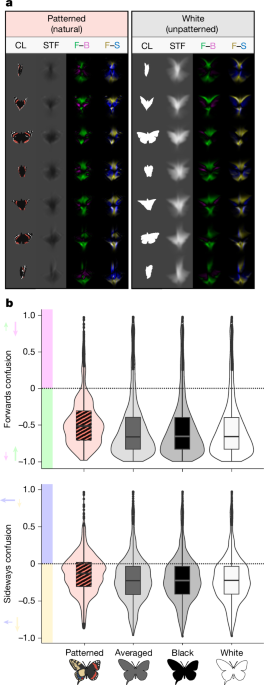
Temporally fluid motion measuresTo quantify the influence of butterfly wings and their patterns on motion detection, we used a custom-written biologically informed EMD28,45, using ImageJ. The model operates using spatiotemporal correlation of pixel intensity values across consecutive frames, quantified with arrays of vertically and horizontally orientated EMDs to measure motion in four cardinal directions (forwards, backwards, left and right)2. This version of the EMD model was first validated in ref. 28, where it was used to quantify high-speed recordings of broadclub cuttlefish Sepia latimanus illusory hunting displays, using the temporal and spatial resolution of green shore crabs, Carcinus maenas.For our model, videos were first processed by spatially and temporally filtering contrasts not visible to the viewer to create ‘fluid motion vision’. Spatial contrast limits were based on those of small passerines (about 6 cycles per degree) observing at 34 cm (smallest) to 193 cm (largest) away, depending on the size of the butterfly. Avian spatial acuity scales with eye and body size46, so these viewing parameters should scale allometrically with larger or smaller predators and butterflies. Temporal limits were chosen based on a 100-Hz critical flicker fusion frequency for a passerine within a forest habitat46,47. We chose these distances to be as biologically realistic as possible: they are close enough to the target that an avian predator would be likely to initiate their ballistic attack. Closer distances are challenging to model, as they require very high frame rates to avoid motion artefacts (this viewing distance already required simulations at 2,000 fps). Meanwhile, longer viewing distances lead to the stripes no longer being resolvable, and are therefore irrelevant for the current hypotheses and attack ranges.Filtering was achieved by interpolating frames and pixels using temporal (σ = 5) and spatial (σ = 8) Gaussian blur. Temporal blurring at σ = 5 reduced a 100-Hz flashing stimulus recorded at 1,000 Hz to 1% of its original amplitude28. In the absence of both spatial and temporal filtering, EMD outputs would have been strongly influenced by temporal aliasing resulting in ‘wagon wheel’-type motion artefacts that would not occur in nature35. The model then outputs motion energy values in each direction (forwards, backwards, left and right) for every pixel and for each consecutive pair of frames.To quantify motion confusion, the strength of motion in each direction was measured as the mean energy across each frame giving a measure of forwards, backwards, left and right energy. To measure how wing patterns ‘confuse’ motion detection relative to the dominant direction of movement (forwards), we calculated Michelson’s contrast of motion for backwards compared with forwards (forwards confusion), and for sideways compared with forwards (sideways confusion)29. Sideways motion was measured using the mean of left energy and right energy.$$\begin{array}{l}\mathrm{Forwards}\,\mathrm{confusion}=(\mathrm{Backwards}\,\mathrm{energy}-\mathrm{Forwards}\,\mathrm{energy})\\ \,/(\mathrm{Backwards}\,\mathrm{energy}+\mathrm{Forwards}\,\mathrm{energy})\end{array}$$$$\mathrm{Sideways}\,\mathrm{energy}=(\mathrm{Right}\,\mathrm{energy}+\mathrm{Left}\,\mathrm{energy})/2$$$$\begin{array}{l}\mathrm{Sideways}\,\mathrm{confusion}=(\mathrm{Sideways}\,\mathrm{energy}-\mathrm{Forwards}\,\mathrm{energy})\\ \,/(\mathrm{Sideways}\,\mathrm{energy}+\mathrm{Forwards}\,\mathrm{energy})\end{array}$$Forwards confusion gives an estimation of how patterning alters the perceived speed of a moving object, with greater values indicating a greater weighting of motion backwards compared with forwards and a slower speed. For most forwards-moving objects the Michelson’s contrast of backwards to forwards energy should be negative, with biological motion such as flapping wings and running limbs generating cyclical periods of greater backwards compared with forwards energy, for example, when a limb swings backwards. Sideways confusion gives an estimation of how patterning alters the perceived turning rate of an object, with greater values exaggerating or dampening turns. Forwards energy on its own can also mislead observers, with more contrasting objects, such as white, resulting in overestimation as opposed to underestimation of object speed by humans48,49. Failure to accurately evaluate the speed or turning rate of an object can result in failure to intercept a target50.It is noted that, for the free-flight videos and the videos presented to human ‘predators’, the direction of the EMD measures did not always align with the heading of the butterfly and was instead globally aligned to the start and end point of the butterfly’s flight path. Meanwhile, for all measurements using the European butterfly simulations and genetic algorithm, the butterfly’s orientation always aligned with the four EMD directions.High-speed analysis of butterfly take-offTo pilot whether and how butterfly wing patterns influence early-stage motion detection of their flight, we recorded the take-offs for five Euro-African butterfly species, two of which were recorded for dimorphic sexes, giving a total of seven morphotypes. These were: Anthocharis cardamines (males, N = 2), Hypolimnas misippus (males, N = 3 and females, N = 3), Papilio dardanus ochracea (males, N = 3 and females, N = 2), Papilio machaon (unknown sex, N = 2) and Vanessa atalanta (unknown sex, N = 3). For H. misippus and P. d. ochracea, the females are mimics of aposematic species of the subfamily Danainae51,52. We recorded take-off behaviour as most predator attacks begin on stationary butterflies. All butterflies filmed were adults, with sample sizes determined by availability. As data collected were based on EMD measurements of take-offs, no randomization was required.Butterfly take-offs were recorded against a green-screen background with a scale bar and Xrite colour checker using a CHRONOS 1.4 (Kron Technologies). The butterflies were typically oriented with their dorsal surface patterning facing the camera. Footage was taken in RAW format at a framerate of 1,057 fps and a resolution of 1,280 × 1,024 pixels. Each species was recorded two or three times (see above for the number of listed flights). Videos were converted from RAW to a DNG stack using the Python function pyraw2dng; these could then be imported into ImageJ and saved in a .tif format. Weka trainable segmentation followed by manual screening and adjustments was used to cluster the video, replacing the background with a dark colour and the butterfly patterning with up to a maximum of four colours53. Each video was cropped to include only the area of the flight path and so that the final frame had the entirety of the butterfly visible. Video durations ranged from 174 to 399 frames (0.16 s to 0.38 s)Once clustered, videos were converted from standard RGB space to avian luminance using blue-tit double-cone quantum catch54,55,56. The background area for each video was replaced with the average luminance for a grassy background (RGB 87, 87, 87). Videos were re-oriented and cropped in length such that the first and last position of the butterfly would follow a linear vertical line upwards (up = forwards) and the butterfly was entirely in frame for its final position. Each video was then passed through the temporally fluid EMD using the methods described above. For each consecutive frame pair, the forwards-confusion and sideways-confusion metrics were calculated using the measured forwards-, backwards-, left- and right-motion energy (Supplementary Video 1). This process was repeated for each video with the butterfly wing patterns replaced with the averaged luminance of the butterfly, 0% reflectance (black) and 100% reflectance (white), giving a total of 4 pattern treatments: natural, averaged, black and white.European butterflies were caught with a butterfly net in a private garden in France (Mareil-Marly, 78750), housed temporarily in individual plastic pots with airholes and filmed outdoors in a netted enclosure. To film the take-off, the pot was placed upside down in front of a green screen and lifted off once the butterfly had settled on the lid; the butterfly was then allowed to take off naturally. Butterflies were released immediately after recording. African species (H. misippus and P. d. ochracea), raised from captive-bred pupae, were filmed using a similar set-up; these butterflies were held using soft tweezers, then released for take-off.Motion confusion across European butterfliesTo assess which features of butterfly wing patterns influence early-stage motion detection of butterflies in flight, we opted to use controlled three-dimensional simulations of European butterflies in flight.Scanning butterfly imagesTo capture the breadth of European butterfly species, we scanned pages from Collins Butterfly Guide as JPEGs using a Konica Minolta bizhub C368 office scanner (Konica House)57. As we were interested in patterning more than exact colour values, the accurately scaled illustrations of butterflies within the guide provided an invaluable resource with dorsal images of 397 butterfly species and a total of 757 unique morphotypes (subspecies and sexes).For each scanned page, individual butterfly dorsal images were cropped and saved in .tif format using a custom-made ImageJ script to semi-automatically select regions of interest for the right forewing and hindwing, as well as a line for the body length. Regions-of-interest selections allowed for later quantification of butterfly wing pattern and shape measures, and for extraction of the forewing, hindwing and body as .pngs for our three-dimensional simulations45. Each scan was saved with a scale of 23.583 pixels per millimetre.Three-dimensional rendering in BlenderTo simulate flight for the European butterfly morphotypes, we constructed a three-dimensional animated model of a butterfly in Blender 4.0 (Supplementary Video 2). The butterfly consisted of five two-dimensional planes: the body, two forewings (left and right) and two hindwings (left and right). The image of each plane could be replaced with one of the avian double-cone catch converted scans for the butterfly’s body, hindwing and forewing. These planes were rigged with an armature for the forewings and hindwings used to generate flapping flight. The wings were animated symmetrically to match the clap and fling flight of one of the videoed H. misippus, with the wings deforming, rolling and yawing distally during the upstroke and downstroke, as opposed to simply pitching upwards and downwards. When animated, the butterfly would fly forwards linearly from its start frame to the end, carrying out two wingbeat cycles.A custom-written ImageJ + Python script was then used to automatically replace the images used for the butterfly’s body, hindwings and forewings with those of a selected butterfly, as well as to adjust the wingbeat frequency and render the animation58. Across Lepidoptera, a smaller wing area corresponds with a higher wingbeat frequency25,59. Higher wingbeat frequencies are likely to interact with how patterning influences motion detectors, resulting in increased motion blur. Wing area for each butterfly was converted to the estimated wingbeat frequency in hertz using an equation calculated from the near-linear relationship between butterfly mass, wing area and wingbeat frequency (see Supplementary Information, section 2 for formula calculation)60:$$\begin{array}{c}{\rm{W}}{\rm{i}}{\rm{n}}{\rm{g}}{\rm{b}}{\rm{e}}{\rm{a}}{\rm{t}}\,{\rm{f}}{\rm{r}}{\rm{e}}{\rm{q}}{\rm{u}}{\rm{e}}{\rm{n}}{\rm{c}}{\rm{y}}\\ \,=\,{10}^{(-0.134346\times ((\log (\text{wing area (}{\rm{m}}{{\rm{m}}}^{2}))/\log (10))\times 1.23952-7.843389)+0.53418)}\end{array}$$The calculated wingbeat frequency was then used to rescale the length of the animation and adjust the start and end frame so that the animation consisted of one wingbeat cycle with ten additional frames lead-in and lead-out for fluid frame interpolation. When rendered, butterflies were filmed from a static bird’s-eye view (camera looking down on the butterfly), flying forwards at a speed proportional to its body length and wingbeat frequency (speed = length × 1.93 × wingbeat frequency). We used only one viewing angle for both tractability and because we did not have access to ventral surface patterns for most of the butterfly species illustrated in Collins Butterfly Guide. Animations were rendered as a stack of .pngs at a frame rate of 2,000 frames per second.Each stack was imported into ImageJ and quantified using the temporally fluid EMD, taking the average forwards, backwards, left and right energy across each frame. These were used to calculate the forwards confusion, sideways confusion and forwards energy for a butterfly in flapping flight. Each butterfly was rendered with three colour treatments: its natural pattern (natural), the averaged grey value of the wing (grey) and in white to account for the effect of the wing shape alone. Natural patterns were used for the random forest analyses, whereas the grey and white renders were used exclusively for linear model comparisons of patterned versus unpatterned butterflies (Supplementary Information, section 2). In addition, each colour treatment was rendered with and without wingbeat animations to determine how gliding influences motion, giving a total of six treatments. This process was carried out for all 757 morphotypes.Butterfly wing featuresTo assess which features of butterfly wings influenced our EMD model, we quantified the colour, patterning and wing shape of butterflies using image analysis. All measures used were repeated separately for the forewing and the hindwing. Simple measures of colour were obtained by converting the butterfly scans to the CIE 1976 Lab colour space61. This colour space is frequently used for the measurement of biological coloration and allows for the quantification of colour across three discrete image channels, L* (achromatic luminance), a* (opponent red–green) and b* (opponent yellow–blue). For each image, we measured the mean and standard deviation (contrast) of a*, b*, and of the Euclidean distance of the a* and b* channels from zero (saturation).For patterning, we used Gabor filters set to 6 different orientations (0°, 30°, 60°, 90°, 120° and 150°) and 6 octaves, the largest being 1/4× the wavelength of the wing (square root of wing area) to measure the pattern contrast, size and orientations of our blue-tit double-cone catch images62,63. The resulting stack of 24 images were then used to create spatial maps for periodicity (how big the pattern is), absolute energy (how contrasting the pattern is), direction encoded as two separate channels VH (0–90 | vertical–horizontal) and OA (135–45 | obtuse–acute), as well as the directionality (anisotropy = √(VH2 + OA2) − average energy; Supplementary Information, section 2). These five maps (periodicity, energy, VH, OA and directionality) allowed us to quantify pattern variation across the wing, not just the global average. For each map, we measured the pixel mean, standard deviation, horizontal gradient (x) and vertical gradient (y). For instance, a high positive mean VH would indicate a vertical rather than a horizontal (negative) pattern, a positive horizontal gradient for periodicity would indicate that periodicity increases distally from the body, and a high standard deviation of directionality would indicate that directionality varies substantially across the wing.Lastly, butterfly size and wing shape were measured by calculating the total wing area, the estimated wingbeat frequency and the body length. Forewing and hindwing shape measurements were made by recording the length of the wing from the centre of the wing base to the most distal point on the wing64, the breadth of the wing at the centroid of the line for the length of the wing, the rectangular length and width of the wing, the area of the wing relative to the body length (area/body length), the aspect ratio of the wing (length/breadth), the circularity of the wing (4π(area/perimeter2))45, and the roughness of the wing (the convex area/the actual area). Altogether, this gave us 73 measures for wing features.In silico butterfly pattern evolutionThe diversity of butterfly wing patterns is a product of unique genetic and developmental pathways, some of which have been accurately mapped4,65,66. These could either limit the adaptive potential of their patterning for motion confusion or could create patterns that fit our motion-confusion hypothesis by coincidence. To validate whether our motion-confusion metrics corresponded with actual butterfly wing evolution, we opted to simulate evolution and selection for motion confusion with genetic algorithms67,68. Genetic algorithms provide a powerful tool for exploring the fitness landscape of animal phenotypes, and have seen increasing use within visual ecology research, notably for animal camouflage research69,70,71. These algorithms mimic evolution by natural selection to efficiently explore vast multidimensional solution spaces, such as those of animal patterns.For the algorithm, we modified the existing animal pattern evolution framework of the CamoEvo Toolbox, which utilizes decimal encoding of reaction-diffusion patterns and subsequent image modifications to produce artificial animal patterns, with mutation operators tailored for the evolution of patterning71. This framework was altered to produce images of artificial butterflies where the parameters for pattern shape were separate for the forewing, hindwing and body of the butterfly, allowing for them to evolve independently from one another. As with the real European butterflies, the butterfly images were then transferred to Blender and animated with our three-dimensional butterfly rig.To account for any influences wing shape might have had on evolution, we selected three distinct butterfly wing shapes from three of the butterfly families: the proportionally small wings of a ‘Skipper’ Hesperiidae (Pyrgus andromedae), the distinct tailed wings of a ‘Swallowtail’ Papilionidae (Papilio machaon) and the more classically shaped wings of a Nymphalid butterfly (Pseudochazara anthelea)72. For each wing shape, we assigned populations of N = 24 butterflies to one of three different measures of ‘fitness’ representing different selection pressures: forwards confusion, sideways confusion and forwards energy. For each generation, the top-8 individuals (that is, those with the highest motion-confusion and energy metrics) would ‘survive’, whereas the remaining 16 ‘died’ and were replaced by mutant recombinant offspring of the survivors in 2 rounds of random pairings. In addition, we evolved butterflies under random selection, where the rank order was randomly generated each generation: this was done to ensure that butterflies did not evolve patterns simply because of drift. Each population evolved for 20 generations, starting with a population of randomly generated individuals, and with 10 repeats for each fitness metric per wing shape, giving a total of 120 populations (3 wing shapes, 4 selection pressures and 10 repeats).Butterflies were expected to become ‘fitter’ with each generation, and to select for similar features to those identified to predict motion confusion in real butterflies. As high-spatial-frequency patterns and speckles were not under selection owing to spatial filtering from our fluid EMD model, both the patterns of real butterflies and the genetic-algorithm-generated in silico butterflies underwent Gaussian spatial filtering (σ = 8) before measurement. For both sets of butterflies, we used the same wing pattern metrics as the European butterfly analysis, excluding measures of wing shape or CIE Lab colour. We chose to use population sizes of 24 individuals and 20 generations based on previous applications63,71 and as we wished to determine the most immediately selected characteristics and to preserve diversity for motion confusion, rather than determine the peak optimum phenotypes.Behavioural validation of measuresTo test whether or not our motion-confusion metrics could predict changes in predator-attack behaviour, we constructed a high-framerate (240 Hz) touch-screen butterfly capture game using the three-dimensional butterfly rig used for the in silico evolution and analysis of scans from Collin’s Guide to Butterflies. This involved the following: subselecting butterflies that were representative of different levels of motion confusion; rendering the butterflies onto 10 different flight paths to create animations for a touch-screen game; and recruiting 100 volunteers to collect data on how motion-confusion measures before the player touching the screen influenced where they clicked relative to the butterfly.For the game, we sub-selected five butterfly phenotypes from the range of Collins Guide to Butterflies. These butterflies were selected from across the motion-confusion gradient for forwards and sideways confusion: Brintesia circe (male), Papilio alexanor (female; it is noted that this species has the highest sideways confusion), Pyrgus sidae (male), Gonepteryx cleobule (male) and Lycaena tityrus (female). See Supplementary Information, section 4 for full table.Butterfly animation and flight behaviourAs with the Collins and genetic-algorithm simulations of butterflies, we used Blender to create artificial renderings of butterflies. Butterflies were re-scaled so that they had the same wing area. Butterflies had a mean body length of 2.42 cm when rendered on the screen. Wingbeat frequencies were adjusted based on body size and wing area, as with our previous simulations. However, unlike the previous simulations, butterflies were animated with an average flight speed of approximatley 40 cm s−1 for a period of 1.458 s, with multiple wingbeat cycles per flight and sinusoidal flight paths, to simulate natural flight behaviour and make them more difficult to capture. Butterflies initiated their flight from the bottom-left corner of a 1,280 × 720 pixel background image, which was the same colour as the previously used backgrounds (RGB 87, 87, 87) and would then fly off the screen either from near the bottom-right or top-right corners. The start position of the butterflies was offset from the centre point in a 50° arc (±25°) centred on 45° from the left corner of the background (Supplementary Fig. 25).As the flight paths were encoded using waves and differences in starting orientation, we were able to create saveable flight paths that could be efficiently stored and used across different butterfly phenotypes. For more details of how the sinusoidal flight was encoded, see Supplementary Information, section 4. We randomly generated 50 flight paths and then sub-selected 5 paths where the endpoint was in the top-right corner and 5 where the endpoint was in the bottom-left corner. The five selected paths for each end point were uniformly selected from low to high levels of linearity (inverse of the level of displacement from the straight-line path from start to end). The settings of each of these paths were saved as .json files, which could be reloaded using Blender and Python, allowing the butterfly phenotypes to be mapped to the same motion paths. See Supplementary Fig. 26 for illustrations of each flight path.EMD measurements and hitboxesButterfly videos were rendered at a frame rate of 1,000 fps and then underwent temporal motion smoothing with the same Gaussian blur levels used for the EMD analyses. As birds see faster than humans, and pilot experiments found that human participants struggled to catch butterflies moving faster than 50 cm s−1, we opted to create targets that flew across the screen at 40 cm s−1, but had the equivalent wingbeat frequency and blur to a butterfly travelling at double the speed 80 cm s−1, which was in the range of speeds for our free-flying butterfly take-offs. This was achieved by resampling the number of frames and then dividing the wingbeat frequency by two for the Blender render before applying the blurring method (Supplementary Fig. 27).After applying temporal smoothing, we downsampled the number of frames to match the frame rate of the monitor, 240 fps, for the game (Supplementary Information, section 4(v)) For each flight path and each phenotype, a second video was rendered using a labelled hitbox created for the butterfly’s image. This hitbox was colour-coded such that the red channel could be used to indicate whether a butterfly was hit (butterfly = 255 R), and the green channel could indicate which region of the butterfly was hit (body = 10 G, forewing = 200 G, hindwing = 255 G or tail = 30 G).For each butterfly and for each path, we measured EMD using the same method of alignment as the butterflies filmed in free flight. The images were re-oriented so that the start and end points were in a straight vertical line upwards. The forwards (up), backwards (down), left and right EMD were then used to calculate the confusion measures (forwards and sideways confusion) for the butterflies. This gave us the EMD and confusion measures for every frame. As confusion varied throughout the flight for each butterfly owing to differences in wingbeat cycle and heading (Supplementary Fig. 28), we created a measure for the mean EMD values and confusion values starting from 400 ms (96 frames) before each frame. However, it is worth noting that changes in the orientation of the butterfly will have resulted in noise in the motion-confusion measures, as they were not always aligned with the direction of movement. For instance, forwards confusion was on average higher for P. alexanor than B. circe, probably owing to movements perpendicular to the start and end heading.Butterfly gameFor the experiment, we recruited 100 anonymous volunteer players from across the University of Exeter’s Penryn Campus (Penryn, Cornwall, UK, TR10 9FE) to play a touch-screen-based butterfly-catching game. Participants were required to be aged between 18 and 70 years old, with normal or corrected to normal vision (that is, wear glasses if needed). The sex and age of the participants were not recorded.The game was run using an ASUS Aspire Nitro V15 laptop with an in-built NVIDIA GEFORCE RTX graphics card, allowing us to display the game with a secondary screen for our experiment, a graphics-processing-unit-powered 240-Hz ASUS XG32UCWMG gaming monitor. The screen for the experiment was 71 cm wide and 40 cm high, with a maximum resolution of 1,920 × 1,080 when in enhanced frame rate mode. Although the uppermost frame rate of the screen was 480 Hz, we selected a vertical refresh rate of 240 Hz for increased stability.To convert the screen into a touch screen, we used a greentouch infrared frame, placed over the monitor and with a thin (2 mm thick) acrylic sheet cut to fit behind it to protect the screen. Infrared frames allow objects, that is, a participant’s finger, that penetrate the frame to be registered as clicks (Supplementary Fig. 29). Infrared frames are advantageous compared with alternative touch device methods owing to their high response rate >240 Hz and their ability to be paired with almost any screen. This method for high-frame-rate touch screens was based on previous studies73,74. Players were seated on a chair positioned about 50 cm away from the screen and were asked to adjust the height of the screen and to adjust themselves to where they could comfortably reach all four corners of the screen without fully extending their arm, and so that their head faced the centre point of the screen. The mean body length of our butterflies was 2.42 cm, giving an angular width of approximately 2.80° and an angular speed of approximately 58.99° s−1.To create the game, we used MATLAB R2025 along with the Psychtoolbox-3 and a suite of custom functions for initializing the screen and Psychtoolbox and for registering the touch output as clicks, dubbed PECK as they were initially developed for experiments using birds73. As PECK has not yet been released, a stripped version of it including only functions necessary for the experiment has been provided within both our Github and Figshare repositories75.Each player undertook 30 trials rendered at 240 Hz with 6 replicates of each butterfly phenotype. The trials used random flight paths, and each path could be flipped on the x and/or y axis. This gave a total of 3,000 trials across 100 participants. Before each trial, the player was first instructed to click on a white circle positioned in the same corner from which the butterfly would start. This meant that the player’s finger always started behind the butterfly. The butterfly would then immediately appear, and the player would have to ‘attack’ it using a single finger. Once the player touched the screen, the butterfly would pause, and text would appear revealing whether the player had successfully hit or missed the butterfly. If the butterfly’s hitbox was within a 30-pixel radius of the click, it was considered a hit. This was to account for the size of the participant’s finger.Before the experiment commenced, the player was given a series of instructions informing them how to play the game and asking them to use only their dominant hand and one finger when playing the game. Players also did a short tutorial to ensure that they understood the instructions and to ensure that they could catch the butterflies at the speed they travelled in the experiment. This tutorial tasked the player to try and click on butterflies of 3 increasing speeds, 0.5×, 0.75× and 1.0× the speed of the butterfly used in the experiment. To progress to the next speed, the player needed to successfully catch two butterflies at that speed. Players, on average, took 14 ± 6 (mean ± s.d.) trials to complete the tutorial. In addition, during the tutorial, when the player clicked the screen, they were also given information about whether their click was to the front or back and left or right of the butterfly. These trials were not included in the count of 30 experimental trials. During experimental trials, the player was no longer provided with any additional information or instruction. When the screen was clicked, they were only informed on whether they hit the butterfly or not, rather than where they clicked relative to the butterfly.Data collectionFor each experimental trial, we recorded the unique ID assigned to the player, the flight path and butterfly phenotype used, the order number of the trial, whether the path was flipped on the x and/or y axis, the coordinates and frame of the touch/click if there was one and the RGB values of the nearest pixel of the hitbox to the click. By using the heading of the butterfly, we were able to calculate the angle of the click relative to the butterfly and the distance of the click on different vectors, the distance parallel to the butterfly’s (y vector) heading and the distance perpendicular (x vector). As click distances were defined relative to the butterfly headings, the y vector was allowed to be positive or negative, with negative values indicating clicks behind the centre of the butterfly and positive values being in front.Statistical analysesAll statistical analyses were carried out using R version 4.3.376.To determine how wing pattern influenced the motion-confusion metrics for real butterfly take-offs in free flight, we used linear mixed models (LMMs), with the ‘lme4’ package77. For the analysis, the motion-confusion metrics (forwards confusion, sideways confusion and forwards energy) were considered as dependent variables in separate models, with wing pattern type (natural, averaged, black and white) as a factorial predictor variable. The ID number for each unique flight and the species were used as random effects. To compare differences between the factor levels, we used emmeans Tukey post hoc comparison tests78.Given the vast array of wing features measured, we opted for a random forest model to evaluate the predictive value for each of the measures for each of our motion-confusion measures33. Random forest provides a non-parametric ensemble learning method, using multiple constructed decision trees trained with random subsets of the data and the predictors. Predictions are then aggregated across the trees helping to prevent overfitting. For each of our metrics, random forest models were trained with 1,500 trees with 4 predictors per split. To evaluate model performance, we used R2 to estimate the proportion of explained variance.Recursive feature elimination was used to improve model interpretability by reducing redundant predictors. Predictors were systematically ranked based on their weight and model performance was evaluated for subsets from one to the total number of variables. R2 values of the complete model and the reduced models were compared to ensure that the predictive accuracy was retained. To evaluate which features of the reduced model were the most important, we used Shapley additive explanations (SHAP) as a measure of feature importance79. Greater absolute SHAP indicates a greater importance, with positive and negative values corresponding with a positive or negative correlation, respectively.Random forest models were performed using ‘randomForest’ and ‘caret’ packages33,80. As many of the wing features are potentially linked to phylogeny, we incorporated the complete European butterfly phylogeny of Wiemers et al. into the model72. Cophenetic distances were extracted from the phylogeny and converted into three phylogenetic principal components with principal coordinate analysis using the ‘phytools’ package81. Similar to how principal component analysis can reduce multiple numeric variables into singular components, principal coordinate analysis allows an individual’s position within the phylogeny to be redefined as a set of multidimensional coordinates. Our three phylogenetic components were included alongside the wing parameters as predictor variables within our model. Circular coordinates for the butterfly phylogeny were extracted with the ‘ape’ package82.For the in silico butterflies, LMMs were used to validate whether butterflies significantly improved in fitness between the first and last generation for each of our selection variables (forwards confusion, sideways confusion and forwards energy) for our evolution treatments. Random forest models were again generated for the motion-confusion metrics using our reduced set of spatially filtered wing pattern variables. These models were created using the measured phenotypes from the first and last generation of the entirety of our in silico-generated dataset, rather than for butterflies under one selection pressure, using the initial randomly generated butterflies to provide a wider range of variation. Lastly, to determine whether or not butterflies under a particular selection pressure evolved to be more or less like the 757 natural butterfly morphotypes scanned from Collins, we generated principal components for the same wing pattern metrics used for our real butterflies, barring measures of colour as the artificial butterflies were rendered only in the luminance channel, (PC1 and PC2) and used pairwise comparison to calculate the Euclidean difference of principal components between every butterfly, both real and in silico, from every natural butterfly.Instances where real butterflies of the same morphotype were compared were removed as their distance would equal 0. Butterflies were divided into 6 groups: natural, forwards-confusion selected (gen = 20, top 1 per population), sideways-confusion selected (gen = 20, top 1 per population), forwards-energy selected (gen = 20, top 1 per population), random selection (gen = 20, top 1 per population) and unevolved (gen = 0, all individuals). We then used a linear model to test which group generated the lowest difference from real butterflies and whether the pairwise distance levels were significantly different from one another with Tukey post hoc comparisons. We hypothesized that the difference should be lower for those selected for motion confusion than for those that were randomly generated at the start.To test whether or not our motion-confusion measures influenced how the butterflies were clicked relative to the butterflies for our behavioural validation, we used an LMM, with the vector distance as the response variable and the axis (x or y) and the predicted motion-confusion measures, forwards confusion, sideways confusion and the forwards energy, of the butterfly as the predictor variables, with the player ID, the trial order and the path ID as random effects, in addition to frame rate as during some trials frame rate dropped to about 220 Hz. For the model, we included interactions between the axis and each confusion measure. Our expectations were that forwards confusion should influence the click distance parallel to the butterfly (y) and that sideways confusion should influence the click distance perpendicular (x).In addition to the linear model, we used two-dimensional kernel density estimation with the Mass package for our vectors to determine how the butterfly phenotypes influenced the shape of the distribution of clicks68. We extracted the grid for the top-25% densest regions of clicks for each butterfly and used ellipse statistics (centroid coordinates, angle, aspect ratio, major and minor width) to describe the shape of where players tended to click. We also used a binomial generalized LMM with the same random effects as the linear model to test whether our EMD measures influenced the likelihood of clicking forewing or hindwing. Clicks to the body and misses were excluded from this analysis.For each model, continuous predictor and response variables were re-scaled to a mean of 0 and a standard deviation of 1.Ethics statementUse of butterflies for flight recordings was approved by the University of Exeter ethics committee (application number eCORN000385). For the behavioural validation game, volunteers were recruited via email and by signs, with ethical approval from the University of Exeter ethics committee (REF: 9474868) and in line with the Declaration of Helsinki. No identifying data were collected as part of the experiment. All volunteers were required to read through the information sheet and sign a copy of the participant consent form. Copies of these forms are available within our data repository75.Reporting summaryFurther information on research design is available in the Nature Portfolio Reporting Summary linked to this article.