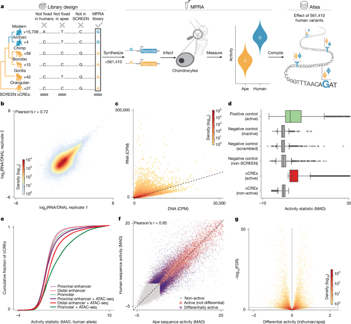
MPRA designLibrary designTo generate the catalogue of fixed human-derived substitutions we used genotyping data from 139 non-human great apes15,68,69,70,71 (10 bonobos, 59 chimpanzees, 43 gorillas and 27 orangutans), all mapped to the human reference genome GRCh37. To restrict the analysis to high-confidence genotypes, we excluded variants that did not meet any of the following criteria: DP ≥ 5 or DP ≥ sample 2.5% percentile, DP ≤ 100 or DP ≤ sample 97.5% percentile, GQ ≥ 20, allelic balance ≥ 0.75 for homozygous calls or between 0.25 and 0.75 for heterozygous calls. In addition, to reduce false positives arising near indel calls, we excluded variants located within ±10 bp of an indel.To generate a catalogue of substitutions that are likely to be derived and fixed in humans, and fixed for the ancestral allele in all non-human great apes, we performed the following filtering steps. First, to include only positions that are fixed in the human population, we used substitutions that are completely (100%) fixed for the human reference allele in 19 human individuals from the great ape catalogue15,68,69,70,71 and do not have an alternative allele in any of the 15,708 human genomes in gnomAD v.2.1.1 (refs. 16,72; we then validated the variant frequencies in additional datasets, see below). Overall, 99.9963% of positions had at least 1,000 genotyped individuals (read coverage > 5). Second, we restricted the analysis to sites fixed (100%) for the non-human allele across all non-human great ape samples with genotypes passing the above filters. Only positions with valid genotypes in at least 80% of individuals of each group (Pan, Gorilla and Pongo) were kept. Multi-allelic alternative variants were excluded as well. Third, to retain variants shared across all human groups, including Neanderthals and Denisovans, we further filtered the dataset by using the variant call files generated using the four high-coverage archaic genomes and excluding sites at which any archaic humans carried an alternative allele17,18,19,20 using standard parameters (removing indels; keeping FILTER = ‘PASS’ or ‘.’; DP ≥ 10; QUAL ≥ 20; GQ ≥ 20). Fourth, for technical limitations in downstream synthesis and cloning, we excluded variants overlapping RepeatMasker repetitive regions (‘low complexity’, ‘simple’ and ‘satellite’ repeat types)73, and simple tandem repeats from Tandem Repeats Finder74, both downloaded from the UCSC table browser75. Finally, we excluded variants overlapping the ENCODE set of problematic genomic regions76. This resulted in a catalogue of 5,731,772 single-nucleotide variants.We validated the frequencies of all variants using two datasets. First, in gnomAD v.4.0 (ref. 16), we found that 80.5% of the variants remained completely fixed in humans, 99.96% had a frequency higher than 0.999 and 99.99% had a frequency higher than 0.99. Second, we used a combined dataset of the 1000 Genomes Project (1KG) and the Human Genome Diversity Project (HGDP), downloaded from gnomAD v.3.1 (ref. 16). This dataset enables a more accurate estimation of global allele frequency. Here, 96.8% of the variants were completely fixed, 99.91% had a frequency higher than 0.999 and 99.99% had a frequency higher than 0.99.Libraries of this size are beyond the current capacity of lentiMPRA. Thus, we further filtered the catalogue for substitutions within candidate cCREs. To this end, we used SCREEN (v.2), the ENCODE project’s database of cCREs defined by chromatin marks21. SCREEN contains 926,535 cell-type-agnostic cCREs, calculated on the basis of 839 human tissues and cells. Elements with the following classifications were included: (1) enhancer-like cCREs; (2) promoter-like cCREs; and (3) DNase-H3K4me3 cCREs, which together cover 7.62% of the genome. This filtering increases the likelihood that a sequence is active by threefold12. This resulted in an initial within-cCRE catalogue of 472,528 substitutions.On the basis of this variant list, we designed a library of 270-bp DNA sequences centred around substitutions in the catalogue. To reduce pool size, adjacent substitutions (≤170 bp apart) were synthesized in the same sequence, centred midway between the outermost substitutions. If additional substitutions fell within the first or last 50 bp of a sequence, they were also included. However, these substitutions (i) did not affect the centring, and (ii) to control for potential edge effects associated with substitutions located near the boundaries of the synthesized sequence, an additional construct centred on each such flanking substitution was designed. Regardless of the number of substitutions in a sequence, each sequence was synthesized twice: once with the great ape ancestral sequence and once with the full set of human-derived substitutions (including substitutions outside SCREEN elements). Sequences overlapping repetitive or problematic regions by more than 25% were excluded. This resulted in a library of 343,503 sequence pairs covering 524,751 substitutions, each represented by its ancestral and derived versions. Because this number exceeds the capacity of a single lentiMPRA, we randomly divided the library into nine sublibraries of around 80,000 sequences. To minimize potential batch effects between sequence pairs, we included both alleles of each sequence within the same sublibrary.A tenth sublibrary included two groups of sequences. First, to take into account promoter strand-specific regulation77, the 5,942 sequences (2,971 sequence pairs) that overlapped with promoters of genes on the minus strand were resynthesized in their native reverse orientation. Promoters were defined as regions ± 500 bp away from a transcription start site (TSS)78. Sequences overlapping promoters of both plus-strand and minus-strand genes were treated as plus-strand sequences.Second, substitutions in CpG islands79 were underrepresented in the original library owing to lower sequencing coverage in the ape genomes. To rescue them, we relaxed the minimum percentage of individuals with a valid genotype required per species group from 80% of all individuals to 30% of individuals with high CpG island coverage in each species group. This translated to 22% in Pan, 20% in Gorilla and 12% in Pongo and added 45,798 sequences (22,899 sequence pairs). Owing to PCR limitations observed in the other nine libraries, sequences with a GC content lower than 43% were excluded. In total, among genomic positions annotated as cCREs by SCREEN v.2 (ref. 21) (7.62% of the genome), 13.98% did not pass genotype quality control, 1.90% overlapped repetitive or problematic regions and 2.54% were located near indel calls. After accounting for overlaps between these regions, 15.59% of the cCRE genomic territory was excluded. The remaining 84.41% was retained for identification of human-derived substitutions. Overall we synthesized 366,402 sequence pairs containing 561,410 single-nucleotide substitutions (Supplementary Table 1).Analyses were performed using BEDTools80, VCFtools81 and BCFtools82. Unless otherwise mentioned, we used GRCh37 as the reference genome in all analyses. The UCSC liftOver tool was used to lift over coordinates between genome assemblies83.MPRA controlsTo estimate the quality of the experiment, and to compare performance across sublibraries, each sublibrary included the following set of controls (Supplementary Table 1). (1) Positive controls for regulatory activity included: (i) 138 sequences previously shown to be active in a published lentiMPRA performed in osteoblasts, the cell type most closely related to chondrocytes (100 of those were also found to be active in embryonic stem cells and/or neural progenitor cells)12; and (ii) 12 previously validated CREs active in chondrocytes84,85,86,87,88,89. In total, there are 150 positive controls for activity in each sublibrary. (2) Negative controls for activity: (i) 100 sequences showing no activity in any of the three tested cell types (including osteoblasts) in a previous lentiMPRA12; (ii) 100 scrambled sequences, generated by randomly shuffling 100 sequences from each sublibrary; and (iii) non-SCREEN controls; that is, 100 sequences centred around human-derived fixed variants that do not fall within SCREEN-defined putative regulatory regions, but do fulfil all other criteria of our library design. In total, we included 300 negative controls for activity in each sublibrary. (3) Positive controls for differential activity: 100 sequence pairs that showed differential activity in a previous lentiMPRA12. In addition, to gain insight into their activity in chondrocytes, sublibrary L3a3 also included the other 307 pairs of differentially active modern-human-derived sequences, allowing all 407 of the reported differentially active sequences to be tested in chondrocytes.MPRA experimentLibrary cloningFifteen-base-pair primer-binding sequences were added to both sides of each 270-bp sequence (Supplementary Table 1), and synthesized in three batches of 240,000 sequences by Twist Bioscience. The tenth sublibrary was synthesized in an additional batch. Each sublibrary was amplified separately by an eight-cycle PCR using sublibrary-specific forward primers (5BC-AG01-f01, 5BC-AG02-f01, 5BC-AG03-f01; Supplementary Table 19) that contain a vector overhang sequence and reverse primers (5BC-AG01-r01, 5BC-AG02-r01 and 5BC-AG03-r01; Supplementary Table 19) that add a minimal promoter (mP) downstream of the test sequence. A second round of nine-cycle PCR was performed with a forward primer (5BC-AG-f02; Supplementary Table 19) and a reverse primer (5BC-AG-r02; Supplementary Table 19) that adds a 15-bp random barcode downstream of the mP. The amplified fragments were then inserted into the AgeI and SbfI sites of the pLS-SceI vector (Addgene, 137725) using the NEBuilder HiFi Master Mix (NEB). The recombination product was electroporated into 10-beta competent cells (NEB) using a Gemini X2 electroporation system (BTX). The transformed cells were cultured overnight on 15-cm 100 mg ml−1 carbenicillin LB agar plates, and the resulting plasmid library was extracted using the QIAGEN Plasmid Plus Midi Kit (QIAGEN). We collected approximately 16 million colonies per sublibrary, yielding an average of 200 barcodes associated with each test sequence.cCRE–barcode associationTo determine the association between barcodes and cCREs, we first amplified a fragment containing the test cCRE, mP and barcode from each sublibrary using primers that contain Illumina flow cell adapters (P5-pLSmP-ass-i# and P7-pLSmp-ass-gfp; Supplementary Table 19). The amplified fragments were sequenced with a NextSeq 550 using custom primers for each sublibrary (R1, pLSmP-ass-seq01-R1, pLSmP-ass-seq02-R1, pLSmP-ass-seq03-R1; R2, pLSmP-ass-seq-ind1; R3, pLSmP-ass-seq01-R2, pLSmP-ass-seq02-R2, pLSmP-ass-seq03-R2; R4, pLSmP-rand-ind2; Supplementary Table 19).The R1 and R3 read pair covered the test sequence and the R2 index read covered the barcode. We obtained at least 60 million reads for each sublibrary. We then used Bowtie2 (ref. 90) to map the read pair covering the test sequence to the original list of 732,804 test sequences, using the preset parameters ‘—very-sensitive’. Next, we kept only read pairs that (i) had the ‘proper pair’ SAM designation; (ii) mapped to the same sequence; and (iii) had at least one read with a mapping quality ≥ 6. After linking each read pair covering the test sequence to the read covering the barcode, we removed barcodes that (i) had a sequencing quality score ≤ 30 for any of the 15 bases of the R2 read; (ii) were associated with multiple sequences; or (iii) had fewer than two independent associations linking the barcode to the sequences. This resulted in a final list of barcode–sequence associations containing 112,470,912 unique barcodes and 684,577 sequences. Data were deposited in the NCBI Gene Expression Omnibus (GEO) under accession number GSE316891.LentiMPRA experimentHuman primary chondrocyte culture was performed according to the manufacturer’s instructions (Cell Applications, 402K-05f). In brief, the cells were maintained in HC basal medium with HC growth supplement. For passaging, cells were dissociated using trypsin and EDTA and plated at approximately 30,000 cells per cm2.Lentivirus packaging was performed as previously described91. In brief, 50,000 cells per cm2 HEK293T cells were seeded in T175 flasks and cultured for 48 h. The cells were co-transfected with (per flask) 7.5 μg of plasmid libraries, 2.5 μg of pMD2.G (Addgene, 12259) and 5 μg of psPAX2 (Addgene, 12260) using EndoFectin Lenti transfection reagent (GeneCopoeia) according to the manufacturer’s instructions. After 8 h, the cell culture medium was refreshed and ViralBoost reagent (ALSTEM) was added. The transfected cells were cultured for 2 days to complete lentivirus packaging. The lentiviruses in the culture medium were concentrated using the Lenti-X concentrator (Takara) according to the manufacturer’s protocol, and resuspended in 1,500 μl phosphate-buffered saline (PBS) per T175 flask. Lentiviral infection, DNA and RNA extraction and barcode sequencing were performed as described previously91. In brief, for each sublibrary, three biological replicates were performed. Eight million chondrocytes were seeded into three 10-cm dishes (2.7 million cells per dish), and cultured for 24 h. Chondrocytes were infected with the lentivirus libraries at a multiplicity of infection (MOI) of 50–100 using ViroMag according to the manufacturer’s protocol. We used 150 μl lentivirus and 220 μl ViroMag per 10-cm dish. Infected cells were grown for 3 days, and total RNA and genomic DNA were extracted using the QIAGEN AllPrep mini kit (QIAGEN). The extracted RNA was purified using the TURBO DNA-free Kit (Thermo Fisher Scientific) and reverse-transcribed into cDNA with SuperScript IV (Thermo Fisher Scientific), using a barcode-specific primer containing a unique molecular identifier (UMI) (P7-pLSmp-ass16UMI-gfp; Supplementary Table 19). Barcode fragments were amplified from both genomic DNA and cDNA, with three-cycle PCR using the UMI primer (P7-pLSmp-ass16UMI-gfp; Supplementary Table 19) and a primer that contained a sample index sequence (P5-pLSmP-5bc-i#; Supplementary Table 19). A second round of PCR was performed to amplify the library using primers containing flowcell adapters (P5 and P7; Supplementary Table 19). The barcode fragments were purified using Ampure XP (Beckman Coulter), pooled and sequenced with NextSeq 15PE using custom primers (R1, pLSmP-ass-seq-ind1; R2 (read for UMI), pLSmP-UMI-seq; R3, pLSmP-bc-seq; R4 (read for sample index), pLSmP-5bc-seq-R2; Supplementary Table 19).MPRA processingBarcode RNA and DNA sequencing and processingPer sublibrary, 50–110 million reads were sequenced for DNA and 120–320 million reads for RNA (data deposited in the NCBI GEO under accession number GSE316891). We aligned the R1 and R3 reads to the barcode–sequence association list using Bowtie2 (ref. 90) with the preset parameter option ‘—very-sensitive’. Next, we applied quality filters to the alignment. We kept only read pairs (i) that had ‘proper pair’ SAM designation; (ii) in which both reads had a mapping quality ≥ 20; and (iii) in which CIGAR string and MD Flag showed a perfect match (15M and 15, respectively). Finally, we removed PCR duplicates by collapsing reads on the basis of UMIs.Some cCREs with multiple barcodes had one or more barcodes with extreme RNA read counts compared with the other barcodes of the same cCRE allele. Such outliers are likely to be due to hyperactive integration loci, and do not represent the true endogenous activity of the cCRE. To minimize such cases, we removed barcodes that had an RNA count higher than or lower than two standard deviations from the mean RNA barcode counts per cCRE allele, as described in our MPRA quality-control pipeline23. On average, 3.58% of barcodes were removed per replicate (324,822 in total; 4.39 per cCRE).Quantifying activityWe used the R package MPRAnalyze22 (v.1.9.1) to analyse the MPRA data. We provided UMI-collapsed read abundances for each barcode as input. To determine which cCREs were capable of promoting expression, we used the RNA and DNA models of the quantification framework of MPRAnalyze (rnaDesign = ~1 and dnaDesign = ~replicate) and extracted alpha, the transcription rate, for each cCRE. MPRAnalyze uses the activity of the scrambled sequences as a baseline against which to estimate the expression level of each tested cCRE. We corrected the mean absolute deviation (MAD) score-based P values from MPRAnalyze for multiple testing across tested cCREs in all sublibraries, excluding any controls and cCREs with fewer than five DNA counts, using the Benjamini–Hochberg method92, thus generating a MAD-score-based activity FDR for each cCRE. We defined cCREs as capable of driving expression (active) if they had an FDR ≤ 0.05. As an additional measure of activity, we calculated a simple ratio of expression as RNA abundance normalized to DNA abundance (RNA/DNA ratio). To do so, we aggregated UMI-collapsed read abundances across all barcodes of each cCRE, separately for DNA and RNA. We then added pseudocounts (+1) to the resulting RNA and DNA counts. Next, we used counts per million (CPM) normalization to correct these counts according to library size. Finally, we divided the normalized RNA counts by the normalized DNA counts. We repeated this calculation for each replicate separately and for the combined outputs of all replicates. Overall, we identified 65,576 active cCREs (Supplementary Table 2).Quantifying differential activityWe used the comparative framework of MPRAnalyze22 to measure differential activity between the human and great ape alleles. MPRAnalyze uses information across all the barcodes for both alleles of a given cCRE, as well as information across all replicates (note that because of run-time issues for the sequence pair seq325030, which had the highest number of barcodes in its sublibrary (10,933), we randomly subsampled approximately half (5,486) of the barcodes for this specific pair. For all other sequence pairs, we used information from all barcodes). To reflect the design of our experiment, we included barcode, allele and replicate information in the DNA model and allele information in the RNA model (rnaDesign = allele, dnaDesign = replicate + barcode_allele, reducedDesign = 1). The differential activity analysis included all cCREs in which at least one of the alleles was defined as active (see above), as well as the active positive and negative controls for differential activity. Then, we extracted the MPRAnalyze P values and differential activity estimate (fold change) of the human relative to the great ape allele. Using the Benjamini–Hochberg method92, we corrected the P values of all sublibraries for multiple testing (excluding controls). We defined all cCREs with FDR ≤ 0.05 as differentially active. Overall, we found 15,077 differentially active cCREs (Supplementary Table 4).Chondrocyte ATAC-seq and CUT&TagATAC-seq was performed in two biological replicates following the manufacturer’s protocol (Tagment DNA Enzyme and Buffer Small Kit; Illumina) with modifications. In brief, the 500,000-chondrocyte cell pellet was washed with PBS and resuspended in 50 μl lysis buffer to isolate nuclei. The nuclei were pelleted and resuspended in 50 μl of a transposition reaction mixture containing 25 μl Tagment DNA buffer and 2.5 μl Tagment DNA enzyme, then incubated at 37 °C for 30 min. Tagmented DNA was purified using the MinElute reaction cleanup kit (QIAGEN).CUT&Tag was performed in two biological replicates using the Hyperactive In-Situ ChIP Library Prep Kit (Vazyme) according to the manufacturer’s protocol, with minor modifications. In brief, 500,000 cells were washed with 250 μl wash buffer and resuspended in 50 μl wash buffer. Cells were incubated with 5 μl of ConA beads for 5 min and collected using a magnet stand. The ConA-bound cells were resuspended in 50 μl antibody buffer and incubated with an anti-H3K27ac antibody (ab4729, Abcam) at 4 °C overnight. Cells were then collected using a magnet stand and further incubated with goat anti-rabbit IgG (ab6702, Abcam) at room temperature for 2 h. Cells were then washed twice with wash buffer and incubated with pA-Tn5 at room temperature for 1 h. After two additional washes, cells were incubated in tagmentation buffer at 37 °C for 1 h to activate tagmentation. The tagmented DNA was treated with 5 μl of 0.5 M EDTA, 1.5 μl of 10% SDS and 1.25 μl Proteinase K, followed by phenol–chloroform extraction and ethanol precipitation.The tagmented DNA extracted from ATAC and CUT&Tag was size-selected twice using 0.65×/1.8× SPRIselect (Beckman Coulter) according to the manufacturer’s protocol. Library amplification was performed as previously described93. The amplified libraries were further purified twice with SPRIselect and quantified on a TapeStation using the High Sensitivity D1000 kit (Agilent).The ATAC-seq and CUT&Tag libraries were pooled and sequenced on an Illumina NextSeq platform to generate 80-bp paired-end reads using a Mid Output 150-cycle kit. Sequencing quality was assessed with FastQC v.0.12.1 (http://www.bioinformatics.babraham.ac.uk/projects/fastqc/). Adapter sequences were removed and reads were quality-trimmed using fastp v1.0.1 (ref. 94) with default parameters. Trimmed reads were aligned to the GRCh38 reference genome using bowtie2 v.2.5.1 (ref. 90) with the following parameters: –very-sensitive –dovetail -I 0 -X 700. PCR duplicates were removed using Picard MarkDuplicates v.3.0.0 (http://broadinstitute.github.io/picard). Peaks were called using MACS3 v3.0.1 (ref. 95) with the following parameters: -f BAMPE -g hs –nomodel –qvalue 0.05.Data have been deposited in the DDBJ database under accession number PRJDB40123.TF-binding sitesWe compared two versions of each variant in the library: one containing the reference human allele and the other containing the alternative (great ape) allele. Each cCRE was associated with potential binding TFs using two independent approaches: find individual motif occurrences (FIMO) and protein binding microarray (PBM). For this analysis, we used only TFs that have been shown to be expressed in chondrocytes (that is, with gene transcripts per million (TPM) > 1)96. The code used for this analysis has been deposited at https://github.com/GokhmanLabOrganization/differential-TF-binding.git.Predicted-motif-based approach (FIMO)Position frequency matrices were downloaded from JASPAR97 as MEME files (JASPAR2024_CORE_vertebrates_nonredundant_pfms_meme). For TFs with multiple reported motifs, we selected a single representative motif using the following prioritization scheme. (i) Motifs derived from in vitro assays (SELEX, HT-SELEX, CAP-SELEX, SMiLE-seq or PBM) were prioritized over in vivo chromatin immunoprecipitation followed by sequencing (ChIP–seq)-derived motifs, ensuring that comparisons were either between in vitro and ChIP–seq or within the same platform. (ii) When multiple motifs originated from the same assay type, we selected the one supported by the highest number of input sites used to determine the motif in the original study (‘nsites’). (iii) If nsites were identical (for example, closely related alternatives such as C/G versus CG), we selected the longer motif.For each variant, we extracted the surrounding sequence and generated reference and alternative allele versions. Sequence length was set by the longest motif in the .meme file, ensuring that the variant is centred and all motif positions are covered. The sequences were written to a FASTA file and analysed with FIMO40 using the following command: fimo –text –thresh 1e-4.FIMO reports scores only for statistically significant matches, but allele comparisons require scores for both sequence versions. Therefore, when a significant match was detected for one allele and the other was missing, we added the corresponding sequence and recalculated binding scores for all sequences to ensure consistency. Scores were computed using the same PWMs as in the .meme file, summing position-wise contributions across the sequence following FIMO’s logic. Significance was assessed by comparing each score with background sequences, with P values defined as the fraction of background scores that were greater than equal to the observed score. We confirmed that this approach reproduces FIMO’s scoring with high correlation. Finally, for each variant, we computed the differential binding score as the human allele version motif score minus the ancestral motif score (because FIMO output scores are expressed in a logarithmic scale).Experimental binding data (PBM)We further used PBM data to quantify TF–DNA interactions. For each variant, we generated all possible 8-mers spanning the variant in every position (eight sequences in total), extracted their binding intensities from PBM data (PBM median fluorescence values) and calculated the differential binding in the same way as for FIMO.The PBM 8-mer data were taken from UniPROBE98 and CIS-BP99, downloaded from the NCBI GEO under accession number GSE53348. We retained pairs in which at least one 8-mer had a median intensity > 0.35. P values were derived from corresponding z-scores and then corrected for multiple comparisons (q-values). Scores with q > 0.05 were discarded, and only allelic pairs passing this filter for both alleles were used for differential binding analysis.TF statistical analysisData were filtered to include only cCREs with a single variant to avoid confounding effects from multiple variants. Fisher’s exact test was used to test for the enrichment of TF-binding sites in differentially active cCREs versus all active cCREs. For each TF, a contingency table was constructed with the categories: TF binding/differential activity; TF binding/no differential activity; no TF binding/differential activity; and no TF binding/no differential activity. Odds ratios and P values were calculated for each TF, and P values were adjusted for multiple testing using the Benjamini–Hochberg FDR correction.Pearson’s correlation coefficients were calculated between differential TF binding z-scores and cCRE fold change (ln), for cCREs with significant differential activity. P values were adjusted for multiple testing using FDR correction (Benjamini–Hochberg method).Human accelerated regions and quickly evolved regionsSome sequences have been shown to evolve rapidly along the human lineage. These include human ancestor quickly evolved regions (HAQERs)100 and human accelerated regions (HARs)101,102. So far, the majority of accelerated regions with known functional effects have been associated with neural processes103,104, but a few have been implicated in skeletal phenotypes13,105. We found that only six HARs contain fixed human-derived substitutions and intersect with active chromatin marks, and none show differential activity. HAQERs, however, show an enrichment in differentially active sequences (2.84×, P = 0.0195, two-sided Fisher’s exact test), suggesting that the emergence of HAQERs might have been associated with shifts in gene regulation, in line with results in neural100 and skeletal13 tissues.Association of MPRA cCREs with target genesTo predict the genes linked to each cCRE, we used five approaches (Supplementary Table 9). (i) Overlap with promoters: we defined promoters as the region 5 kb upstream to 1 kb downstream of NCBI GRCh37 transcripts106, and assigned each cCRE to all the promoters in which it fell. (ii) Proximity to a TSS: because many CREs preferentially affect their nearest gene107,108,109, we linked each cCRE to its closest TSS. (iii) Proximity to known eQTLs: we used GTEx eQTLs and their associated genes from all tissue types110, and intersected eQTLs with our set of cCREs. We linked each cCRE to the target gene(s) of any eQTL within ±1 kb. (iv) Spatial interaction with a promoter: we used high-throughput chromosome conformation capture (Hi-C) to map spatial interactions between the cCREs and their target genes. To this end, we used Hi-C data111,112,113 from chondrocytes and mesenchymal stem cells, as a close proxy for chondrocytes. We intersected each cCRE with the promoters it interacted with, up to ±1 kb away. (v) Association with eRNA: eRNAs have been shown to be significantly co-expressed with the promoters they regulate114. Thus, if a cCRE overlapped an eRNA-expressing locus, we associated it with the genes co-expressed with that eRNA. We downloaded FANTOM5 eRNA data115 from GeneHancer31, which contains a list of eRNA coordinates and their associated genes.To enrich for cCRE–gene links that are relevant to chondrocytes, we retained only links to genes expressed in chondrocytes by using two datasets from the ENCODE portal116 (https://www.encodeproject.org/) with the following identifiers: ENCSR000CUE and ENCSR774MGO. We defined genes as expressed if they had an expression level higher than 1 TPM). After combining both datasets and their replicates, we defined 14,206 genes as expressed in chondrocytes.For analyses in which the cCRE–gene associations should be particularly reliable (enrichment analyses, and selection of top candidates; see below), we used a stricter subset of cCRE–gene associations that we termed ‘elite associations’. Elite associations were defined as cCREs either that are located within the promoter of a gene, or where at least two independent methods agreed on the same target gene.Functional enrichment analysesGenes associated with differentially active cCREs using elite associations (n = 1,280; Supplementary Table 10) were tested for functional enrichment using GO33, the HPO database34 (release 2024-04-26) and the GAD35. To control for potential biases arising from factors such as variant choice, MPRA design or the genomic distribution of SCREEN elements, we used as background all genes linked to active cCREs (n = 9,975; Supplementary Table 10). Thus, the test and background gene sets differed only by whether their variants alter gene activity. Differential activity was defined using a minimum threshold of |FC| > 1.333; cCREs below this threshold were treated as active but non-differentially active and included in the background set. Hypergeometric test P values were calculated for each term. To reduce multiple-testing burden, terms associated with fewer than 20 differentially active genes were excluded. For HPO enrichment, we used only phenotypes related to the skeletal system, as defined by Gene ORGANizer117.Similarly, we ran an enrichment analysis on the set of 4,463 human-derived differentially expressed genes, comparing them to the set of expressed, but non-differentially expressed, genes. The IPA enrichment analysis was run on version 159584291, 6 May 2026. Input included the set of 4,463 human-derived differentially expressed genes along with their fold change and FDR-adjusted P values for differential expression.GAG biosynthesis selection analysisWe defined GAG-related genes as those associated with any of the four GAG metabolic pathways in KEGG38. This included 73 genes related to GAG synthesis (hsa00532, hsa00534 and hsa00533) or degradation (hsa00531). For simplicity, in Fig. 3d, we show only genes related to the synthesis of the linker or chain region. Genes related to sulfation patterns were not included. Dermatan sulfate was not included, because it does not bind to aggrecan37. For keratan sulfate, only KSII (O-linked) biosynthesis was included, because it is the mode of glycosylation in aggrecan118.The lineage-specific selection test was performed by comparing the cCREs associated with the 73 GAG genes described above with other cCREs. We first defined a set of cCREs that met three criteria: (i) were significantly active; (ii) had a minimum of 50 barcodes for both the ancestral and human-derived alleles; and (iii) were linked through elite associations to genes expressed in chondrocytes. This yielded a total of 40,941 cCREs. Of these, 11,700 active and 2,768 differentially active cCREs were linked to KEGG pathway annotations38. For cCREs that were active but not differentially active, the ln(fold change) was set to zero. To generate a neutral expectation, we randomized fold-change values across cCREs, while maintaining their gene associations. This procedure was repeated n = 500,000 times. We then compared the observed sum of ln(fold change) associated with each of the four GAG pathways to n random samplings (Srand) of the same number of cCREs affecting the same number of genes. For stringency, we required that each randomized sample include at least one differentially active cCRE. Statistical significance was assessed by computing a P value as the fraction of random iterations in which the sum of ln(fold change) was at least as extreme as the one observed (Sobs) for each pathway, as defined below:$$P=\frac{{\sum }_{i=1}^{n}({S}_{i}^{\text{rand}}\ge {S}_{\text{obs}})+1}{n+1}.$$Cell-type specificity analysiscCREs for 13 cell types were downloaded from SCREEN v.4 on 24 April 2026. We filtered the available SCREEN datasets to the ‘core’ collection. Because the available chondrocyte cell type in SCREEN is in vitro differentiated, we compared it with other in-vitro-differentiated cell types. For each cell type, we computed the correlation of the MPRA-derived cCRE activity (MAD score) with the SCREEN DNase z-score per cCRE. DNase z-scores are normalized DNase accessibility signals, which are comparable across cell types. If several SCREEN elements overlapped a cCRE, we used the cCRE with the highest z-score. We repeated the analysis twice: once for all active chromatin types (promoter-like signature (PLS), chromatin-accessible (CA)-H3K4me3, proximal enhancer-like signature (pELS) and distal enhancer-like signature (dELS)) and once for enhancers only (pELS and dELS) (Supplementary Table 3).Comparing cellular trans environmentsWhereas the human allele was tested in its native human trans environment, the human–chimpanzee ancestral allele was assayed in a human rather than in a human–chimpanzee ancestral trans environment. For an MPRA sequence to exhibit differential behaviour across trans environments, the interacting trans factors must differ—either in their protein sequence (affecting binding affinity) or in their expression levels. We therefore sought to assess these sources of potential divergence.First, we examined evolutionary changes in TF coding sequences that might alter DNA-binding specificity. We used a previous study119 that identified human-specific variants that are predicted to affect TF DNA-binding domains. Notably, only three TFs (ZFAT, ZFHX4 and ZNF18) were implicated. Of these, ZNF18 is not expressed in chondrocytes (TPM 40, we tested motifs for ZFAT and ZFHX4 within our test sequences and found that none of these TFs is predicted to bind to them (FDR > 0.05). This suggests that coding changes between humans and chimpanzees in TF DNA-binding domains are unlikely to make a major contribution to our results.Next, we evaluated differences in TF expression levels between humans and chimpanzees. Notably, human-versus-chimpanzee divergence overestimates human-versus-ancestor divergence, because \(\mathop{5}\limits^{ \sim }\)0% of human-versus-chimpanzee changes are chimpanzee-specific and thus do not contribute to differences between humans and their ancestors. Because expression data from human and chimpanzee chondrocytes are, to our knowledge, unavailable, we analysed cranial neural crest cells (CNCCs)25, which give rise to the facial skeleton. Across TF-encoding genes (n = 736, as defined by JASPAR97), we observed high correlations between species (Pearson’s r = 0.90, P = 1.8 × 10−261, Spearman’s ρ = 0.90, P = 5.2 × 10−272), indicating broadly conserved TF abundance across these skeletal contexts.Because differences in measurements of TF expression between these human and chimp cells are driven not only by genetically encoded changes, but also by technical factors (for example, experimental noise), we turned to investigating TF expression in the human–ape hybrid osteochondral progenitors, which provide a more tightly controlled system for assessing genetically encoded cis-regulatory differences that affect TF genes. We found that TF-encoding genes show a high correlation in these cells as well (Pearson’s r = 0.94, P = 1.1 × 10−276.Finally, we also compared gene expression profiles between human chondrocytes and human osteochondral progenitors, and observed high overall concordance (Pearson’s r = 0.86, P = 2.2 × 10−308), further supporting the notion that closely related skeletal cell types share a similar trans environment.Although these results suggest that most TFs are likely to have similar levels in human and human–chimp ancestor cells, there are nevertheless some differences. Previous studies suggest that such variation affects mainly the magnitude rather than the direction of allelic effects. For example, in our MPRA of modern-human-derived variants in osteoblasts and neural progenitor cells, all allelic pairs (100%) showed concordant directionality of effect across the two cellular contexts12. To further examine this, we analysed our positive control sequences, previously assayed in osteoblasts and here in chondrocytes, and found that 89.52% retained the same direction of differential activity across cell types, and also exhibited a strong correlation in effect size (Pearson’s r = 0.64, P = 2.2 × 10⁻²³).Overall, although the precise contribution of trans differences between a human cell and an ancestral cell to differential activity is difficult to quantify, our analyses suggest that this contribution is limited, particularly with respect to the directionality of allelic effects.GWAS catalogue analysisTo test the overlap of differentially active cCREs with skeletal-related loci, we first generated a list of skeletal-related phenotypes from the GWAS Catalog120 using the following set of keywords and regular expressions: musculoskeletal; skelet(al|on); bone(s)?; cartilage; cartilaginous; ossif.; joint(s)?; arthritis; osteoarthritis; rheumatoid; osteoporosis; osteopenia; fracture(s)?; scoliosis; kyphosis; lordosis; osteonecrosis; osteomyelitis; osteomalacia; osteopetrosis; osteogenesis imperfecta; rickets; spondyl.; ankylos.; gout(y)?; Paget; achondroplasia; chondrodysplasia; chondrocalcinosis; osteochondr.; osteophyte(s)?; intervertebral; disc degeneration; hallux valgus; bunion; osteosarcoma; spine; spinal; vertebra(e|l)?; hip(s)?; knee(s)?; ankle(s)?; elbow(s)?; shoulder(s)?; wrist(s)?; hand(s)?; foot; feet; femur; femoral; tibia; tibial; fibula; fibular; humerus; humeral; radius; ulna; ulnar; pelvis; pelvic; craniofacial; mandible; mandibular; maxilla; maxillary; carpal; tarsal; metacarpal; metatarsal; phalange.*; calcaneus; rib(s)?; bone mineral density; BMD; eBMD; bone area; bone geometry; trabecular; cortical (bone|thickness); heel bone; and quantitative ultrasound. Occurrences of joint(s)? were excluded when followed by statistical-context terms, including analysis, analyses, test, model, modeling, modelling, meta, effect, effects, distribution, study or studies. We then defined 1-kb windows centred on GWAS (genome-wide association study) variants associated with these terms, and tested whether human-derived variants in differentially active cCREs were enriched in these regions relative to other variants in our MPRA library. We found that human-derived variants in differentially active cCREs showed a significant enrichment in skeletal GWAS regions (Fisher’s exact test, P = 0.02).Generation of human–gorilla composite cell lines (hybrid cells)Ethics statementApproval for the derivation of human iPS cell lines used in this study was granted by the University of Chicago institutional review board (IRB) under protocol 11-0524. The human donors in this study consented to the use of their cells (fibroblasts) to generate iPS cells for studies of evolution and cross-species comparisons, and to the generation of other cell types that would be derived from these iPS cells. Donors consented to the deposition of any resulting data from the study in the NCBI GEO. The generation of human–ape composite iPS cells was approved by the Weizmann IRB under protocol 1586-2.We note that these tetraploid cells are not approved for use in vivo or for attempting to generate an organism (which, biologically, is likely to be impossible). We recommend that all future applications of these cells occur in close consultation with bioethicists.Generation and characterization of gorilla iPS cellsGorilla iPS cells were generated by the CRYOZOO biobank of animal cell lines (UPF, EMBL Barcelona, Barcelona Zoo and MCNB) from primary skin fibroblasts using a Sendai virus-based reprogramming approach (CytoTune -iPS 2.0 Sendai Reprogramming Kit, Invitrogen, A16517). Fibroblasts at passage 2 were seeded 2 days before transduction at a density of 5 × 10⁴ cells per well in six-well plates coated with growth-factor-reduced Matrigel (80 μg ml−1) and cultured in αMEM supplemented with 10% fetal bovine serum (FBS), 1% penicillin–streptomycin and 1% GlutaMAX. On day 0, cells were transduced with Sendai viral vectors encoding KOS (human KLF4, human OCT4 and human SOX2), human MYC and human KLF4 at an MOI of 5:5:3, following the manufacturer’s instructions with minor modifications.After transduction, cultures were fed daily with fresh αMEM-based fibroblast medium until day 6. On day 7, cells were passaged at a 1:2 ratio onto Matrigel-coated plates and maintained in αMEM-based medium. Cultures were progressively transitioned from fibroblast medium to mTeSR1, first using a 3:1 fibroblast medium ratio and subsequently to complete mTeSR1 once iPS cell colonies became morphologically distinct. Well-defined iPS cell colonies emerged after approximately 2 weeks in complete mTeSR1. Individual colonies were expanded and maintained on Geltrex (0.16 μg ml−1) in StemMACSiPS-Brew XF medium supplemented with iWR-1 (0.5 μM) and CHIR99021 (1 μM). For cryopreservation, iPS cell cultures at approximately 80% confluence were frozen in FBS containing 10% dimethyl sulfoxide (DMSO).The pluripotent state of the gorilla iPS cell line GiPSC16 was assessed by immunocytochemistry using the StemLight Pluripotency IF Antibody Sampler Kit (Cell Signaling Technology, 9656). Expression of the pluripotency-associated markers OCT4, SSEA4, NANOG, TRA-1-60 and SOX2 was evaluated using the corresponding primary antibodies at a 1:200 dilution. Cells were washed twice with PBS and fixed with 4% formaldehyde for 20 min at room temperature. For detection of intracellular and nuclear antigens, cells were permeabilized with 0.1% Triton X-100 in PBS for 10 min and washed three times with PBS. Non-specific binding was blocked with 1% bovine serum albumin (BSA) and 0.1% Triton X-100 in PBS for 30 min. Cells were incubated with primary antibodies diluted in blocking buffer for 1 h at room temperature or overnight at 4 °C. After three washes with PBS, cells were incubated with the appropriate species-specific Alexa Fluor-conjugated secondary antibodies (Abcam) at a 1:200 dilution for 2 h at room temperature in the dark. Anti-rabbit IgG secondary antibodies were used for OCT4, NANOG and SOX2, whereas the corresponding anti-mouse secondary antibodies were used for SSEA4 and TRA-1-60. Cells were subsequently washed three times with PBS, and nuclei were counterstained with DAPI (0.1–1 μg ml−1) for 1 min.Functional pluripotency was further assessed by directed differentiation of GiPSC16 into derivatives of the three embryonic germ layers using the Human Pluripotent Stem Cell Functional Identification Kit (R&D Systems, SC027B), according to the manufacturer’s instructions. Lineage identity was evaluated by immunocytochemical detection of SOX17 (endoderm), OTX2 (ectoderm) and brachyury (mesoderm), using the primary antibodies supplied with the kit at a final concentration of 10 μg ml−1. After incubation with primary antibodies, cells were incubated with the corresponding Alexa Fluor-conjugated anti-goat IgG secondary antibodies (Abcam) at a 1:200 dilution for 2 h at room temperature in the dark. Nuclei were counterstained with DAPI. Fluorescence images were acquired using a Leica TCS SP8 confocal laser-scanning microscope.Cell fusionBefore cell fusion, 4 to 5 × 10⁶ human (H21792)121 and gorilla iPS cell lines were thawed in 2 ml Dulbecco’s PBS (DPBS; Sartorius, 020201A) supplemented with 5% FBS (Gioco, 12070106). Cells were centrifuged at 1,000 rpm for 5 min, the supernatant was aspirated and pellets were resuspended in 10 ml mTeSR1 Plus medium (STEMCELL Technologies, 100-0274) supplemented with 10 μM ROCK inhibitor Y-27632 (Tocris, 1254/10) and 50 μl penicillin streptomycin (2,500 U; Gibco, 15070063). Cells were seeded onto 10-cm plates coated with Matrigel (Corning, 354277; 1:100 in DMEM/F-12, Diagnobum, D814). The medium was changed after 2 days. On day 3, cells were dissociated with accutase (Sigma, A6964) for 2 min at 37 °C, and dissociation was stopped with DPBS containing 5% FBS. Cells from each line were transferred to separate 15-ml conical tubes and centrifuged at 1,000 rpm for 5 min. The supernatant was aspirated, and cell pellets were resuspended in 10 ml mTeSR1 Plus medium supplemented with 10 μM ROCK inhibitor Y-27632. Cells were counted using an automated cell counter (RWD, C100-SE) and distributed into five 15-ml conical tubes as follows: six million human iPS cells; six million gorilla iPS cells; one million human iPS cells; one million gorilla iPS cells; and a mixed population containing 0.5 million human iPS cells and 0.5 million gorilla iPS cells. Cell labelling and fusion were performed as previously described24, with modifications detailed below. Cells were centrifuged, the medium was aspirated and pellets were resuspended in 2 ml dye solution as follows: human iPS cells were labelled with CellTracker Deep Red (1.5 μM in DPBS; Invitrogen, C34565), gorilla iPS cells were labelled with CellTracker Green CMFDA (5 μM in DPBS; Invitrogen, C7025) and the mixed-cell sample was resuspended in DPBS containing DMSO (1:1,000) only. Tubes were incubated for 30 min at 37 °C with resuspension every 10 min, followed by centrifugation. Dye solutions were aspirated, and cells were washed three times with DPBS. Cells were then plated onto two Matrigel-coated 6-well plates (fusion and control) in 3 ml mTeSR1 Plus medium supplemented with 10 μM ROCK inhibitor Y-27632. Each well of the fusion plate contained one million human iPS cells and one million gorilla iPS cells. The control (no-fusion) plate included one well with unlabelled mixed cells (0.5 million human iPS cells and 0.5 million gorilla iPS cells), one well with one million gorilla iPS cells only, one well with one million human iPS cells only and one well with labelled mixed cells (0.5 million of each). Plates were incubated overnight at 37 °C. Fusion was performed the following day. Medium was aspirated from each well of the fusion plate, and cells were washed twice with DPBS. Polyethylene glycol 1500 (PEG) was added to each well (1 ml per well) and incubated at 37 °C for 2 min. PEG was aspirated, and cells were washed three times with mTeSR1 Plus medium, after which 4 ml mTeSR1 Plus medium supplemented with 10 μM ROCK inhibitor Y-27632 was added to each well. A day after fusion, medium was changed for all the cells (mTeSR1 Plus medium with 5 μM ROCK) and four Matrigel-coated 10-cm plates were prepared. The following day, cells were dissociated with accutase as described above. After centrifugation and removal of DPBS and accutase, cells were resuspended in sorting buffer by pipetting using a P1000 pipette, as described previously25. Cells were then placed on ice before sorting. Cells positive for both Deep Red and Green CMFDA, and negative for DAPI, were sorted using a FACSAria cell sorter into 15-ml tubes containing 2 ml ice-cold DPBS supplemented with 5% FBS (Supplementary Fig. 1). Cells were centrifuged at 1,000 rpm for 5 min, DPBS was aspirated and cells were resuspended in mTeSR1 Plus medium with 10 μM ROCK inhibitor Y-27632 and 2,500 U penicillin–streptomycin. Cells were plated on the prepared Matrigel plates at a density of 10,000 cells per plate. For the following five days, culture medium was supplemented with 5 μM ROCK inhibitor and replaced every two days until colonies became clearly visible. Colonies were picked and transferred, one colony per well of a 12-well Matrigel-coated plate. Each picked colony was assigned a unique identifier (1–96). The medium was replaced every two days, and once colonies reached a sufficient size, each line was passaged into a single well of a Matrigel-coated six-well plate. Cells were maintained under feeder-free conditions until reaching approximately 90% confluency. Each human–gorilla composite cell line was then dissociated using 300 μl accutase, as described above. After centrifugation, cells were resuspended in mTeSR1 Plus medium supplemented with 10 μM ROCK inhibitor Y-27632 and 2,500 U penicillin–streptomycin. A total of 0.5–1 million cells from each line were collected for PCR screening of potential composite cell lines, and the remaining cells were seeded onto pre-prepared 10-cm plates. DNA was extracted from each cell line using the Monarch Genomic DNA Purification Kit (NEB, T3010), according to the manufacturer’s instructions. PCR was performed for each cell line using AR primers specific to human (1,674 bp) and gorilla (536 bp) amplicons. Then, 160 ng genomic DNA from each sample was amplified in a 20-μl reaction containing GoTaq Green Master Mix (Promega, M7122) using a MiniAmp Plus thermal cycler (Thermo Fisher Scientific). Karyotyping was performed on all human–gorilla composite cell lines exhibiting both human and gorilla PCR bands by G-banding, following standard procedures122.Differentiation into osteochondral progenitor cellsDifferentiation of human–gorilla and human–chimpanzee composite iPS cells into limb osteochondral progenitor cells was performed as described123,124, with minor modifications. In brief, iPS cells were counted and seeded at 9,000 cells per well in triplicate onto Matrigel-coated 24-well plates (10 μl ml−1 in DMEM, at least 1 h at 37 °C) and cultured for 24 h in mTeSR1 (STEMCELL Technologies, 85850) supplemented with Y-27632 (Tocris, 1254, 10 μM) and penicillin–streptomycin (25 IU ml−1). Medium was replaced with mTeSR1 containing penicillin–streptomycin without Y-27632, and cells were cultured for an additional 48 h. After DPBS washing, cells were cultured for 24 h in mid-primitive streak (MPS) medium prepared as described123,124. To accommodate rapid cellular expansion, an additional split point was introduced at this stage. Cells were dissociated by accutase (BioLegend, 423201) and replated onto Matrigel-coated 12-well plates in lateral plate mesoderm (LPM) medium, followed by 24 h of culture. Cells were washed with DPBS, the medium was replaced with limb bud mesenchyme (LBM) medium and cells were cultured for 48 h. LBM cells were washed with DPBS and dissociated with accutase, and viable cells were counted. A total of 90,000 cells per well were seeded onto fibronectin-coated (R&D Systems 1918-FN, 4 μg ml−1 in DPBS, 1 h at 37 °C) six-well plates. The medium was replaced after 48 h, and cells were collected 24 h later and snap-frozen in liquid nitrogen, to be used for RNA extraction.RNA extraction and sequencingRNA was extracted by detaching the entire well using accutase, followed by centrifugation at 200g for 5 min. The supernatant was aspirated, and the resulting cell pellet was immediately plunged into liquid nitrogen to prevent RNA degradation. The RNeasy Mini Kit (QIAGEN, 74104) was used according to the manufacturer’s instructions. The RNase-Free DNase Set (QIAGEN, 79254) was applied to the membrane during RNA extraction according to the manufacturer’s instructions. RNA purity and concentration were assessed using a NanoDrop spectrophotometer. Three samples out of ten underwent an additional clean-up step following the manufacturer’s instructions. RNA concentration was quantified using the Qubit RNA Assay Kit (Qubit RNA BR Assay kit, Q10210) and measured with a Qubit 3 Fluorometer. RNA integrity was assessed using the Agilent 2200 TapeStation System by an external service provider. Two technical replicates from each sample were submitted for RNA-sequencing library preparation using TruSeq Stranded mRNA, following the manufacturer’s instructions. Library preparation was performed by the Crown Genomics institute of the Nancy and Stephen Grand Israel National Center for Personalized Medicine, and sequencing was performed on an Illumina (NovaSeq X Plus 1.5B) platform, generating approximately 160 million paired-end reads per sample (2 × 150 bp).For clarity, we use the term osteochondral progenitor cells and not expandable limb bud mesenchyme123, to provide a biological rather than a technical interpretation for these cells’ identity, as previously described123,125. We further validated this identity by a principal component analysis (PCA) (Extended Data Fig. 6b), and by confirming expression of the osteochondral markers SOX9, PRRX1 and absence of NANOG expression (Supplementary Table 8), as described125. Data have been deposited in the NCBI GEO under accession number GSE316892.Identification of gene expression differencesWe used the allele-specific expression pipeline adapted from a previous study25. The whole pipeline was done twice independently using human (GRCh38) and chimpanzee (panTro6) reference genomes for human–chimpanzee hybrids, and human (GRCh38) and gorilla (gorGor6) reference genomes for human–gorilla hybrids. The alignments were performed using STAR (v.2.7.11b) with arguments: -outSAMattributes MD NH -outFilterMultimapNmax 1 -sjdbGTFfile -sjdbOverhang 149. Two-pass mappings were performed (with the option –sjdbFileChrStartEnd to specify the splice junctions identified in the first round of mapping) to improve alignment accuracy. Duplicate reads were removed using Picard v.2.18.27 with the argument DUPLICATE_SCORING_STRATEGY = RANDOM. The set of single-nucleotide variants used to assign reads to either the human or chimpanzee genome was generated as previously described27. The human–gorilla single-nucleotide variant set was constructed using a similar approach, excluding filtering for single-nucleotide variants identified as homozygous in the human and gorilla parental lines. To minimize potential allelic imbalance biases when aligning one species to the genome of another species, we used a modified version of WASP126 (https://github.com/TheFraserLab/Hornet). In this pipeline, only reads that are mapped to the same position after in silico allele swapping are kept, thus ensuring that the variants in themselves do not create biased read mappability. Reads overlapping indels were also discarded. Read count data have been deposited in the NCBI GEO under accession number GSE316892.To compute differential gene expression between human and chimpanzee, and between human and gorilla, we used DESeq2 (ref. 127). We used the likelihood ratio test and the model cond_Cell+cond_Species, in which cond_Cell represents the replicates and cond_Species represents the species. The analysis was done twice, first with counts derived from alignment to the GRCh38 reference genome, and then with counts derived from alignment to the panTro6 or gorGor6 genome. P values were adjusted for multiple testing using the Benjamini–Hochberg false discovery rate. Log2-transformed fold change (log2FC) estimates of human versus ape were shrunk following the recommendations of the DESeq2 workflow128. A gene was classified as differentially expressed between the pair of species only if it met all of the following criteria: (i) it was annotated in both genomes; (ii) it showed significant differential expression when reads were aligned to the human reference, and again when they were aligned to the non-human ape reference genome; and (iii) the log2FC values of differential expression when aligned to the human and non-human ape reference genome were in the same direction and differed by no more than 1.In the osteochondral progenitor human–chimpanzee composite cell lines, differentially expressed genes were classified as human-derived if the gorilla allele expression level (TPM) in the osteochondral human–gorilla hybrid cells was closer to the chimpanzee TPM than to the human TPM. Conversely, genes were classified as chimpanzee-derived if the gorilla TPM was closer to the human TPM than the chimpanzee TPM (Fig. 2d). For this purpose, we did not require the human–gorilla difference to be significant.Detection of aneuploidyTo identify potential aneuploidy, we tested for species-biased stretches of deviations of the log2FC values along each chromosome using a Mann–Whitney U-test. In the osteochondral progenitor human–chimpanzee hybrid cells, we found a bias towards the human allele in the long arm of chromosome 20 and a bias towards the chimpanzee allele in the short arm (Extended Data Fig. 11a). For osteochondral progenitor human–gorilla cells, we found a bias towards the human allele in part of chromosome 18 (chr. 18: 43276708–73564699, GRCh38) for both cell lines (HG1 and HG2) and in part of chromosome 1 (chr.1: 150000000–248956422) for cell line HG1. In addition, there was a bias towards the gorilla allele in part of chromosome 14 (chr. 14: 50000000–107043718) in both cell lines (Extended Data Fig. 11b). We therefore removed these sections from all downstream calculations (TPM and differential expression).Differentiation PCAPCA was performed on the combination of a previously published dataset (Yamada et al.123) and our osteochondral progenitor human–chimpanzee and human–gorilla hybrid datasets. Genes with TPM > 1 in at least two samples were used. TPM values were transformed using log2(TPM + 1), and the 1,000 most variable genes in the Yamada et al. samples were selected. To mitigate technical differences between datasets, samples were assigned to batches according to their identifiers (Yamada, human–chimpanzee hybrids or human–gorilla hybrids), and batch effects were regressed out on a per-gene basis using a linear model with batch as a categorical covariate. The resulting residual expression values were then z-scored for each gene across samples using scaling parameters learned from the Yamada et al. dataset. PCA was subsequently fitted on the standardized Yamada et al. expression matrix, and the remaining samples were projected onto the same PCA space.
ACAN GAG anchor repeat analysisTo determine the number of repeat units in ACAN, the repeat unit sequence defined as ‘repeat type 2’ in a previous report45 (GGGCTTCCTTCTGGAGAAGTTCTAGAGACCGCTGCCCCTGGAGTAGAGGACATCAGC) was aligned to 342 long-read de-novo-assembled haploid or diploid genome builds from 158 humans (316 haplotypes)129,130 (Supplementary Table 14) and 20 non-human great apes (26 haplotypes)131,132,133,134 (Supplementary Table 13). Alignments were performed using BLAST+ (v.2.14.0)135 with the following parameters: ‘-task blastn -word_size 7 -evalue 1e-1 -perc_identity 70 -qcov_hsp_perc 80’. In cases in which a genome build was unavailable or when the ACAN locus was poorly assembled, the raw long-read sequences were used instead136,137.Alignment matches were inspected manually, because occasional misclassification of DNA segments led to missed repeat calls. Thus, the number of repeat units was corrected by dividing the genomic span of the detected repeat region by the repeat unit length (57 bp), calculated as the position of the most downstream match minus the position of the most upstream match.Partitioning of human repeat-count distributionTo characterize heterogeneity in the distribution of repeat counts across human haplotypes, we applied model-based clustering using the Mclust function from the mclust R package (v.6.0.0)138. The distribution of repeat counts was modelled as a finite mixture of Gaussian components, with the number of components G ranging from 1 to 5. Model selection was performed using the Bayesian information criterion (BIC), and the model with the highest BIC was selected (G = 2). For each haplotype, model-based posterior classification probabilities were computed, and haplotypes were assigned to the component with the highest posterior probability.Comparison of GAG composition between humans and non-human great apesEthics statementAll tissues were collected post-mortem (Extended Data Figs. 8 and 9 and Supplementary Table 15). No animals were killed for the purpose of this study. Ape specimens were obtained opportunistically after death. Chimpanzee hand samples were obtained from a 60-year-old female individual, who died of natural causes at the Zoological Center in Ramat Gan, Israel on 27 April 2024). Hand specimens were stored at −80 °C and thawed before tissue collection. All other ape specimens were obtained through collaboration with European zoos (call through the European Association of Zoos and Aquaria). All procedures were performed in accordance with approval number M011/2026 from the KU Leuven Ethical Committee of Animal Experimentation.Formalin-fixed human specimens were obtained from the Farkas Family Center for Anatomical Research and Education (CARE), Rappaport Faculty of Medicine, Technion—Israel Institute of Technology. All procedures conformed to the ethical guidelines of the Technion and the Israeli Ministry of Health. Informed consent was obtained from all body donors, explicitly permitting the use of donated tissues for anatomical education and research.Sample collectionHand articular cartilage: articular cartilage samples were collected from human and chimpanzee specimens from the following hand joints: the first metacarpophalangeal joint (MCP; n = 14), the second–fourth MCP joint (n = 21), the proximal interphalangeal joint (PIP; n = 17) and the distal interphalangeal joint (DIP; n = 18). Full-thickness cartilage samples, measuring approximately 0.5–1 cm in maximal dimension depending on joint size and available articular surface, were collected from each site. For joint samples, full thickness was defined as extending from the articular surface to the underlying subchondral bone. A skin incision was made directly over each joint, followed by careful dissection and reflection of surrounding soft tissues to expose the joint capsule. When necessary, the fibrous digital flexor sheath was opened at the level of the annular pulleys to facilitate access to the articular cartilage.Elbow articular cartilage (capitulum): the upper limb was positioned in supination. Skin and subcutaneous tissue over the cubital fossa were reflected to expose the distal arm and proximal forearm. The plane between the brachialis and brachioradialis muscles was dissected to gain access to the elbow joint. After identification of the humeral capitulum, the overlying articular cartilage was collected using a no. 10 scalpel blade.Elbow articular cartilage (trochlea): the upper limb was positioned in supination. Skin and subcutaneous tissues were reflected over the cubital fossa to expose the distal arm and proximal forearm. The brachialis, pronator teres and common flexor tendon were identified and reflected to gain access to the medial aspect of the elbow joint. The medial epicondyle of the humerus was identified as an anatomical landmark, and the humeral trochlea was exposed immediately distal to it. The articular cartilage overlying the trochlea was then dissected using a no. 10 scalpel blade.Knee: medial femoral condyle: the skin overlying the knee was reflected to expose the distal portions of the vastus medialis and vastus lateralis muscles, as well as the superior border of the patellar ligament. A transverse incision was then made at the level of the patellar ligament and extended superiorly along the margins of the vastus medialis and vastus lateralis for approximately 8–10 cm, circumferentially outlining the knee joint. This soft-tissue flap was reflected superiorly to expose the knee-joint capsule. The capsule was incised, and the leg was subsequently flexed to open the joint space and allow clear visualization of the femoral condyles. Articular cartilage was then collected from the medial femoral condyle using a no. 10 scalpel blade.Knee: proximal tibia: the skin overlying the knee was reflected to expose the distal portions of the vastus medialis and vastus lateralis, as well as the superior border of the patellar ligament. A transverse incision was made at the level of the patellar ligament. The soft-tissue flap was reflected superiorly to expose the knee-joint capsule. After capsular incision and flexion of the leg, the proximal articular surface of the tibia was visualized. The menisci and tibial plateau were identified, and articular cartilage was collected from the medial tibial facet using a no. 10 scalpel blade.Shoulder: humeral head: the donor body was positioned prone. The skin over the shoulder and proximal arm was reflected to expose the deltoid muscle and the proximal portion of the triceps brachii. These muscles were then reflected to gain access to the glenohumeral joint region. The humeral head was identified, and the overlying articular cartilage was collected using a no. 10 scalpel blade.Wrist: scaphoid articular cartilage: the distal forearm was dissected to expose the flexor and extensor tendons of the radial aspect of the wrist. The tendons forming the anatomical snuff box—that is, the abductor pollicis longus, extensor pollicis brevis and extensor pollicis longus—were identified and reflected to expose the radioscaphoid joint. On the flexor aspect, the radial artery and the tendon of flexor carpi radialis were identified and reflected to improve visualization of the joint. The articular surface of the scaphoid was then identified, and the overlying cartilage was collected using a no. 10 scalpel blade.Hip: femoral head: an anterior approach was used. The inguinal ligament was identified, and the soft tissues over the proximal anterolateral thigh were dissected from the level of the anterior superior iliac spine distally to expose the trochanteric region of the femur. The femoral head was then mobilized from the hip joint, and the overlying articular cartilage was collected using a no. 10 scalpel blade.All samples were immersed in 1× PBS and stored at 4 °C.DNA quantificationThe DNA content of each sample was quantified using a Hoechst 33258 fluorescence assay. A dye buffer was prepared from 10 mM Tris base, 1 mM EDTA and 0.1 mM NaCl, adjusted to pH 7.4. Hoechst 33258 (Sigma, 94403) was prepared as a 1 mg ml−1 stock solution in distilled water and stored protected from light at 4 °C. Immediately before use, the dye was diluted in dye buffer to a final concentration of 0.1 µg ml−1.Double-stranded DNA standards were prepared in PBS from a 50 µg ml−1 working stock to generate a standard curve ranging from 0 to 6 µg ml−1. Before dilution, the DNA standard (Sigma, D4522) was heated at 100 °C for 10 min. Papain-digested samples (see ‘Sample digestion and DMMB assay’) were diluted in PBS with a 1:25 dilution.Standards and samples were loaded in triplicate into black 96-well plates at 10 μl per well. Hoechst dye solution was then added at 200 µl per well and incubated for 10 min. Fluorescence was measured using excitation at 350 nm and emission at 450 nm. DNA concentrations in the samples were calculated from the standard curve and corrected for dilution (Supplementary Table 20). Correlation between technical replicates was high (Pearson’s r = 0.97, P = 2.5 × 10⁻⁷ (Extended Data Fig. 10a). DNA content was correlated with sample weight (Pearson’s r = 0.70, P = 1.4 × 10⁻²¹ (Extended Data Fig. 10b).DMMB preparationThe DMMB reagent was prepared by dissolving 16 mg DMMB (1,9-dimethylmethylene blue) in 1 l distilled water containing 3.04 g glycine and 2.37 g sodium chloride. The solution was stirred at room temperature protected from light, and the pH was adjusted to 3.0 using HCl before use139.Sample digestion and DMMB assaySamples were weighed, finely minced, and digested in 400 μl papain digestion buffer containing 40 μg ml−1 papain (prepared by diluting a 25 mg ml−1 papain stock; Sigma, P3125) at 65 °C for 48 h. After papain digestion, samples were diluted in 1% (w/v) BSA. sGAG content was quantified using the DMMB assay, with a standard curve generated from chondroitin sulfate sodium salt (Sigma, C8529). Ten microlitres of each sample or standard was loaded in triplicate into a transparent 96-well plate, followed by 200 μl DMMB reagent per well. Absorbance was measured immediately at 525 nm. Standard error per sample ranged between 0.02 and 5.94, with an average of 0.49. Triplicate measurements were averaged to generate a single value representing the sGAG content of each sample. Measurements were normalized separately by two factors: DNA content (see above) and weight. Normalized values for both methods are provided (Supplementary Table 17). The normalized sGAG content was strongly correlated between technical replicates (Extended Data Fig. 10c) and similar to the literature140,141,142,143.Confounder analysis: sexTo test potential confounders, we analysed the effects of age and sex on normalized sGAG content. Sex was not a significant predictor of sGAG content in either humans or apes (Extended Data Fig. 10d). Similarly, no significant effect of sex was detected when each joint was analysed separately (P between 0.116 and 0.687 for joints with three samples or more) (Extended Data Fig. 10e).Confounder analysis: ageWe used two methods to correct ape ages for cross-species comparison: (i) division by maximum observed lifespan per species144 and (ii) a time-translation framework145. To this end, we generated a set of human-to-ape age conversion tables based on a previously published time-translation framework for developmental events145. Using the pipeline provided in the paper, we produced an output table in which each row is an event × species observation. Gestation days per species were taken from the AnAge Database (build 15)144. We converted the post-conception days (DD) values to years after birth using the following function:$${\rm{A}}{\rm{g}}{\rm{e}}({\rm{y}}{\rm{e}}{\rm{a}}{\rm{r}}{\rm{s}})=\frac{{10}^{{\rm{D}}{\rm{D}}}-\mathrm{gestation}\_\mathrm{time}}{365}$$The resulting event–age pairs were sorted and projected onto the closest monotonically non-decreasing curve using isotonic regression (sklearn.isotonic.IsotonicRegression), which removed minor non-monotonicities introduced by imputation noise without distorting the fit. A monotone interpolating curve was then fitted to the isotonic-corrected pairs using a piecewise cubic Hermite interpolating polynomial (PCHIP), with extrapolation disabled.All species PCHIPs were evaluated on a shared dense grid of 2,000 values along Model_Event, restricted to the intersection of their observed event ranges. The resulting paired points (human_age and ape_age) were then used to fit a final per-species linear regression across the full valid range, by ordinary least squares (numpy.polyfit (degree 1)):$$\mathrm{ape}\_\mathrm{age}\,=\,\alpha +\beta \times \mathrm{human}\_\mathrm{age}.$$The linear regression enabled us to extrapolate values beyond the provided range (Extended Data Fig. 10f,g).Similarly to sex, chronological age was not a significant predictor of GAG content in either humans or apes (Extended Data Fig. 10f). Furthermore, using both age-adjustment methods, ape samples consistently showed a higher GAG content than did their adjusted age-matched human counterparts (Extended Data Fig. 10h).Statistical analysisJoint-level testIn cases in which an individual had more than one sample per joint, the mean of the samples was used. After this procedure, 74 data points remained (57 humans and 17 apes). For phalangeal subregions (PIP, MCP and DIP) with a single ape sample, parametric z-score tests were performed. For other joints (wrist, shoulder, hip, elbow and knee) with larger sample sizes, independent two-sided t-tests were used to compare human and ape values. P values were FDR-adjusted using the Benjamini–Hochberg method92.Global (all-joint) testData points were further collapsed to retain a single value per individual. After this procedure, 49 data points remained (42 humans and 7 apes). A two-sided t-test was used to compare human and ape values.Reporting summaryFurther information on research design is available in the Nature Portfolio Reporting Summary linked to this article.