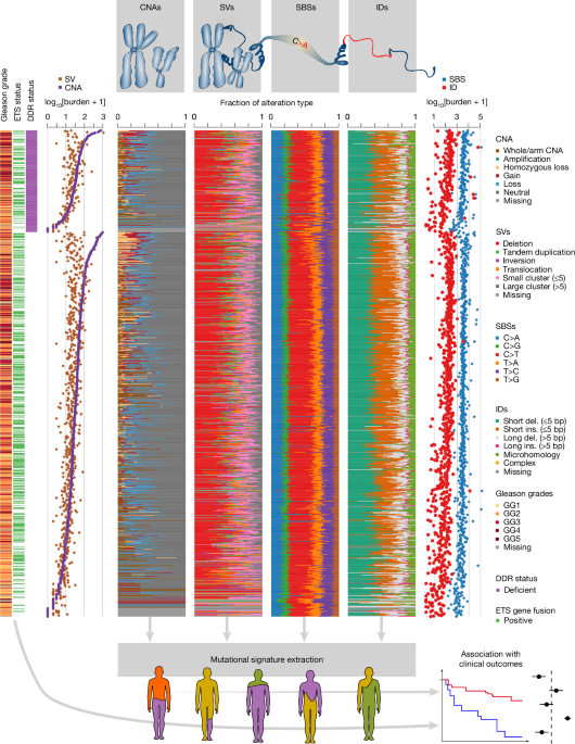
PPCG cohort, WGS and variant callingWe used data from the PPCG consortium of primary prostate cancer samples from a total of 1,001 prostate cancer donors with 1,172 tumour samples. Informed ethical consent was obtained at clinical follow-up, and was consistent with local research ethics and International Cancer Genome Consortium (ICGC) guidelines (https://icgc.org/). Ethical approval was obtained from local research ethical committees (details are provided in the Supplementary Methods).Analysis of SVs from genomic dataSimple and complex SV classification methodWe conducted SV classification on the PPCG cohort using the cSVc tool18, including also SVs near TARBS and chromothripsis, both abundant in prostate cancer. First, exact breakpoint estimation from our WGS short-read sequencing data was conducted by using split-read information. Specifically, for each sample, we used the median of soft-clipped reads from the corresponding tumour BAM file to obtain corrected breakpoint positions. Next, we used ClusterSV18 to obtain clusters of SVs from the corrected SV data and we also used Battenberg68 to obtain segmented CN files from tumour and normal read coverage files. For each sample, we generated CN files segmented by corrected SV breakpoints by using the corrected SV data, the CN segmentation file, CN coverage and the tumour BAM file. Finally, we conducted simple and complex SV classification (chromothripsis excluded) using the CN-SV segmentation file together with the corrected SV file, ClusterSV file and information about ploidy and purity.To classify chromothripsis on the PPCG cohort, we used Shatterseek v.0.4, using SV and CN data. We used Shatterseek’s recommended cut-off criteria to obtain high-confidence calls69. Multiple-testing correction was performed on the P values of three statistical tests indicative of chromothripsis (breakpoint enrichment test, exponential clustering test and the fragment joins test) and we used a q-value cut-off of 0.2 for the chromothripsis calls on each chromosome to confine the final high confidence call set.To obtain the final SV dataset we merged the chromothripsis call set with the remaining simple and complex SV call set. Specifically, we merged calls only if a minimum of 90% of SV call sets spanning the chromothripsis cluster were marked as Complex Unclassified.Tandem duplication detectionThe presence of TDP samples was assessed by using three criteria described previously70. The criteria involve the proportion of tandem duplications, the total tandem duplication count and a TDP score71:$${\rm{T}}{\rm{D}}{\rm{P}}\,{\rm{s}}{\rm{c}}{\rm{o}}{\rm{r}}{\rm{e}}=-\frac{\sum _{i}|{{\rm{O}}{\rm{b}}{\rm{s}}}_{i}-{{\rm{E}}{\rm{x}}{\rm{p}}}_{i}|}{{\rm{T}}{\rm{D}}}$$For a given sample, Obsi denotes the observed tandem duplications for chromosome i, Expi denotes the expected tandem duplications for chromosome i and TD is the total number of tandem duplications. We calculated Expi by counting the tandem duplications per chromosome among all samples and dividing this by the sample size. Together, we classified TDP samples when the following criteria were met: tandem duplication proportion > 20%, total tandem duplication count > 50, and TDP score > −1.Enrichment analysis of SV classes at specific genomic features were performed using a permutation testing framework as described in the Supplementary Methods.De novo extraction and assignment of mutational signaturesSBS and ID signaturesFor the de novo extraction of SBS and ID signatures we considered high-accuracy SNVs and stringently filtered (Tier 1) high-accuracy indels called and quality controlled as described previously24. SBS signatures were extracted de novo using SigProfilerExtractor (v.1.1.23)72. De novo extraction of SBS signatures (96 channels) and ID signatures (83 channels) was performed for 3 to 25 signatures for SBS and 1 to 25 signatures for ID using the following parameters: nmf_replicates=500;nmf_init = “random”;min_nmf_iterations=10,000;max_nmf_iterations=1,000,000;export_probabilities=True;make_decomposition_plots=True;get_all_signature_matrices=True. We then decomposed every set of signatures (3 to 25 signatures for SBS and 1 to 25 signatures for ID) independently to known COSMIC signatures (v.3.4 for SBS and v.3.3 for ID) using the default parameters of the decompose_fit function of SigProfilerExtrator. To find the optimal number of SBS or ID signatures, respectively, we investigated each obtained set of signatures based on a number of features (Supplementary Methods).Structural variant signatures (cSV)We extracted SV signatures by incorporating a non-negative matrix factorization (NMF) framework onto specific feature counts of the SV data. For deletions and tandem duplications, we grouped the SV classes into four different size groups: 0–50 kb, 50–500 kb, 500 kb to 5 Mb and >5 Mb. Each of these groups was further subdivided on the basis of breakpoint occurrence at distinct replication timing regions (early, mid and late) by applying bedtools pairToBed between SV data and replication timing data (see the ‘Enrichment analysis of SV classes at specific genomic features’ section of the Supplementary Information for details about assessment of replication timing status). In the same manner, we also incorporated a group that captured deletions and tandem duplications occurring at fragile sites (see the ‘Enrichment analysis of SV classes at specific genomic features’ section of the Supplementary Information for details about fragile site data). For balanced inversions, and the two local 2-jump classes Dup-invDup and Loss-invDup, we created two groups based on size with a 100 kb threshold. Templated insertion groups (chains, cycles and bridges) were divided by a 5 kb size threshold. Lastly, we included two novel features compared to a previous study18, including chromothripsis and SV breakpoints in close proximity to TARBS, a unique feature of prostate cancer genomes. We counted SV breakpoints occurring at TARBS regardless of SV class (see the ‘Enrichment analysis of SV classes at specific genomic features’ section of the Supplementary Information for details about TARBS data). These groups were converted into a matrix that was used as input for the NMF (NMF package in R)73. For finding the optimal number of SV signatures, we applied a procedure used for finding the optimal number of rearrangement signatures in the Palimpsest R package74. In brief, based on 100 iterations, we determined the index for which the cophenetic values had the steepest decrease and used that index as the number of signatures. We normalized the SV signature values by dividing each value in a row with the row sum and subsequently visualized these values with ggplot2. We also extracted cSVs from WGS data of the HMF-Prostate cohort to quantify cSV signatures (see the ‘Processing genomic data from the HMF-Prostate cohort’ section).CX signaturesCX signatures were identified and quantified from absolute copy-number profiles as previously described17 (Supplementary Methods).We computed the genome-wide distributions of the five fundamental copy-number features for each sample (the segment size, the difference in copy-number between adjacent segments, the lengths of oscillating copy-number segment chains, the breakpoint counts per 10 Mb, and the breakpoint counts per chromosome arm). Feature distributions observed in the cohort were then deconstructed into a total of eight signatures by applying a NMF. All of these signatures were already present in the pan-cancer compendium of CX signatures17 (cosine similarity > 0.85). The final signature activities for all samples were computed using the linear combination decomposition function from YAPSA75 (R package, v.1.12.0) on the feature component-distributions given a predefined signature matrix. To ensure the robustness of the signature activities and to enable trust in small signature activities, we identified signature-specific thresholds by following the same procedure as in our previous work17. We next set activities to zero if they were below the signature-specific threshold. The sample-by-activity vector was finally normalized per sample. This approach was also applied to quantify CX signatures in the HMF-Prostate cancer cohort (see the ‘Processing genomic data from the HMF-Prostate cohort’ section).Identifying integrated mutational footprintsWe performed clustering of patient tumours defined by the complete spectrum of signatures to characterize the main mutational processes driving prostate cancer. For each sample, we combined the activities of each of the different types of mutational signatures into a single vector for clustering input, whereas only signatures being active in any of the clustered samples were considered. The data were scaled and centred before clustering, which was performed independently for samples with CIN and without CIN (non-CIN). Given that all tumours share a core set of clock-like mutational signatures36 complemented with more distinct mutational processes during tumorigenesis, we opted to use hierarchical clustering given the natural hierarchical structure of the data. We tested a broad range of clustering parameters and empirically determined that the Ward-D2 algorithm in combination with Manhattan distance best identified known biological features of our cohort. This approach has also been chosen in other studies76,77 to prioritize robust identification of known biology. In the case of clustering CIN samples, we excluded samples with fewer than 100 SNVs, fewer than 10 indels, or fewer than 5 SVs. We identified eight clusters of CIN samples (Fig. 4b) based on (1) the obtained minimum, median and maximum cluster stability metrics (Supplementary Fig. 12); (2) the silhouette scores in samples (Supplementary Fig. 13); and (3) biological expert knowledge. Each of these clusters characterized a distinct mutational process represented by the integration of mutational signatures. Thus, we referred to these processes as IMFs. In the case of non-CIN samples, we excluded samples with less than 100 SNVs, or less than 10 indels (244 cases; Supplementary Fig. 17). As performed for CIN samples, we explored cluster stability metrics to select 4 clusters for non-CIN samples (Supplementary Figs. 18 and 19).To quantify the activity of the eight IMFs in a given tumour, we first generated an IMF definition matrix, where each IMF was defined across the 46 multi-signature space (22 SBS, 10 ID, 8 CX and 6 cSV signatures). This was done by averaging the multi-signature activities across all samples within each cluster (Extended Data Fig. 6). Then, given the IMF definitions, we applied the linear combination decomposition function from YAPSA75 to the multi-signature vector for each tumour to compute the activity of each of the eight IMFs in the tumour sample. The resulting IMF activity vector is then normalized to sum to 1.After quantifying the activities of the IMFs, each sample was classified according to its dominant mutational process, defined as the IMF with the highest activity. This stratification was applied for testing the potential of the IMF as biomarkers for predicting metastasis occurrence and treatment response (see the ‘Predicting clinical outcomes in cases of primary prostate cancer’ section).Linking mutational processes with genomic featuresHere we performed association analyses between activities of the integrated mutational footprints and different genomic features. We also correlated each individual mutational signature (SBS, ID, cSV and CX signatures) with different genomic features (detailed below). Only samples with available calls for a specific mutational signature and genomic feature were included in each analysis.Spearman’s correlation was applied to test the correlation of IMF activities with the 44 individual mutational signatures. All P values were corrected for multiple testing using the Benjamin–Hochberg method (Extended Data Fig. 7a).Selection of 1,747 genes of interestWe compiled a list of 1,747 genes by integrating and curating the annotations provided in refs. 78,79,80,81. This set of genes included driver genes recurrently altered in prostate cancer21,82, known pan-cancer driver genes, as well as genes reported to be involved in DNA damage response and repair (DDR) pathways, DNA replication, the cell cycle and chromatin organization. For all 1,747 genes, we identified their transcriptional start sites (TSS) on a GRCh37 reference genome using ENSEMBL. We selected the canonical TSS for each gene.Mutation status of genes of interestFor each gene, we integrated germline and somatic alterations for classifying samples as mutant using the following criteria.Oncogenes: samples with amplifications and somatic mutations that did not result in the truncation of the oncogene were classified as mutant. For oncogenes located in autosomal chromosomes (that is, SPOP, IDH1 and MYC), amplifications were considered in cases in which the copy-number value at the transcriptional start site exceeded the sample ploidy by at least two copies. For oncogenes located in sex chromosomes (AR), the threshold was adjusted to require a gain of at least two copies more than the ploidy − 1. Given that the amplification of the enhancer region is frequently observed to be amplified after ADT treatment83, we scanned a genomic region consisting of 0.5 Mb before the TSS and 1 Mb after the coding region of the AR oncogene.Tumour suppressor genes: only samples with biallelic inactivation or homozygous deletion (copy-number value TP53, samples with germline variants or single hotspot driver mutations; (2) for CDK12, samples with single hotspot driver mutations; and (3) for DDR-related genes, samples with germline variants due to its impact on cancer risk. For BRCA1 mutants, we also evaluated the presence of reversion mutations rescuing the HRD phenotype. Rescue was defined by a mutation in either TB53BP1, RIF1 or MAD2L284,85. None of the BRCA1 mutant samples presented reversion mutations.To test for differences in signature activities between samples with and without mutations in any of the 1,747 key genes, we divided the samples into two groups: one group with a mutation and one without. We then used Welch’s t-test to perform a test of equality of means between the two groups. Only positive associations were shown to mitigate compositional data effects. To ensure high-confidence associations, we discarded gene associations lacking a moderate/large effect size (Cohen’s d 4c).In the case of individual mutational signatures, we limited the association analysis to well-known prostate cancer genes21,82, filtered out genes with less than ten samples mutated, and the analysis was performed for the whole cohort and also after stratifying samples on the basis of age at diagnosis (Fig. 2d and Supplementary Fig. 29).Deficiency in DDR mechanismsHere we evaluated differences in signature activity between samples deficient and proficient for five different DDR mechanisms: HR, MMR, NHEJ, NER and BER. To do so, we first evaluated the mutation status of genes involved in each DDR pathway. Samples with inactivation of at least one of the DDR-related genes were classified as deficient; otherwise, as proficient. The genes evaluated for each repair pathway were as follows: HR: BRCA1, BRCA2, PALB2; MMR: MLH1, MSH2, MSH6, PMS2; BER: MUTYH, NTHL1, POLD1, POLE, WRN; NHEJ: NBN, RAD50, ATM; and NER: DDB2, ERCC2, ERCC3, ERCC4, ERCC5, POLD1, POLE, XPC, XPA, CUL3.For each repair mechanism, Welsh’s t-tests were performed to compare signature activities between deficient and proficient samples. P values were corrected for multiple testing using the Benjamini–Hochberg method. Cohen’s d was computed to assess the size of the difference between groups (Fig. 2e, Supplementary Fig. 22 and Extended Data Fig. 7).Assigning mutational signatures to mutationsFor each mutation type in a sample, SigProfilerExtractor72 outputs the posterior probability of a mutation being generated from a signature given the mutation type. The probability is computed by SigProfilerExtractor from the estimated exposure of each signature in the sample, trinucleotide profilers of the de novo extracted signatures, and the abundance of each mutation type in the sample. The SigProfilerMatrixGenerator package was used for classifying SNVs into 96 categories and for classifying indels into 83 categories based on the sequence context86. We then assigned mutations to the signature with the highest probability given their mutation type, as previously done in other studies87,88,89. We note that flat signatures, such as SBS5 and SBS40a, are intrinsically difficult to distinguish because their trinucleotide profiles have low information content and high similarity to one another16,90.WGDTo test whether the WGD status associated with the activity of a signature, we compared activities between samples with and without WGD by applying a Welch’s t-test. Only samples with activities higher than zero were included in the analysis. P values were corrected for multiple testing using the Benjamini–Hochberg method. Cohen’s d was computed to assess the size of the difference between groups (Extended Data Fig. 4b).Whole-chromosome CNAsCopy-number segments were classified as a whole-chromosome alteration if it was larger than 95% of the whole chromosome length covered and had a copy-number value greater or smaller than 2. We then compared signature activities between samples with and without whole-chromosome CNAs using a Welch’s t-test. P values were corrected for multiple testing using the Benjamini–Hochberg method. Cohen’s d was computed to assess the size of the difference between groups.Focal amplificationsFocal amplifications were defined as segments with a copy-number value equal or higher than 8. We then compared the activities of signatures between samples with and without focal amplifications using a Welch’s t-test. P values were corrected for multiple testing using the Benjamini–Hochberg method. Cohen’s d was computed to assess the size of the difference between groups.Microsatellite instabilityMicrosatellite instability (MSI) was evaluated using MSIsensor-pro v.1.3.0 with the default parameters44. In brief, MSIsensor-pro scan was first executed on the reference genome to obtain homopolymers and microsatellites. Next, MSIsensor-pro was applied on tumour and normal BAM files with the homopolymer and microsatellite information file, and with coverage threshold set to 15 and coverage normalization set to 1. Samples with a score higher than 10 were considered as MSI-Hi.HRDetectWe used HRDetect43 to detect the presence of samples with HRD. In brief, we combined all four mutation data type (SV, CNA, SNV and indels) as input for HRDetect to infer six HRD-associated features (microhomology deletions, SBS3 and SBS8 signature, SV3 and SV5 signature). These features were then used to compute an HRD probability score using the default parameters. We considered all samples with a probability score > 0.7 to have HRD.KataegisThe detection of kataegis was performed as described previously24. We counted the number of kataegis events per sample and tested the Spearman correlation to the signature activities. Multiple-testing correction was performed according to the Benjamini–Hochberg method.Cell cycle progression scoresRNA-sequencing (RNA-seq) data were processed and harmonized before downstream analysis as described previously24. For this analysis, we used the high-confidence set of gene expression data (tier 1) RUV-III PRPS-normalized data (v.1.4/K10). Cell cycle progression (CCP) scores, also known as Prolaris scores, were computed for each sample. For each of the 31 genes in the CCP signature63, log2-normalized expression values were centred and scaled relative to the median expression of the specific gene across all samples. The resulting values were then summed to produce a single CCP score per sample. All 31 signature genes were available in the tier 1 data release used for this analysis.AR pathway activitiesThe pathway scores were computed from AR and prostate cancer-related gene sets using the singscore package (https://doi.org/10.18129/B9.bioc.singscore) v.3.21 as described in our companion paper24 using the singscore HALLMARK_ANDROGEN_RECEPTOR as a representation of AR activity.Hypoxia scoresA hypoxia score was computed as described in our companion paper24 using the ‘Buffa’ hypoxia signature91. In brief, the hypoxia score was computed for each RNA-seq sample by median-centring gene expression across the cohort, scaling to unit variance and summing across signature genes to yield a single hypoxia score.ARBS mutation rate enrichmentChromatin immunoprecipitation–sequencing (ChIP–seq) data of prostate tumour-specific AR binding (TARBS, 9,181 sites), normal prostate-specific AR binding (NARBS, 2,690 sites), FOXA1 (19,735 sites) and HOXB13 (66,104 sites) were obtained from ref. 12. TARBS were overlapped with FOXA1 ChIP–seq peaks and HOXB13 ChIP–seq peaks to obtain co-binding sites (Supplementary Fig. 11a). Assay for transposase-accessible chromatin using sequencing (ATAC–seq; 111,884 sites) data were obtained from ref. 92. ATAC–seq peaks were overlapped with TARBS to obtain TARBS+ ATAC–seq sites. ATA–seq peaks without TARBS overlap were sampled without replacement by selecting sites that match the ATAC–seq signal of each TARBS+ ATAC–seq site—this forms a set of TARBS− ATAC–seq sites with matching site number and ATAC–seq signal distribution for comparison to TARBS+ ATAC–seq sites (Supplementary Fig. 7c). Similarly, TARBS were downsampled to match the number and ATAC–seq signal of NARBS for an additional validation (Supplementary Fig. 7b). Chromatin state data were obtained from ref. 34. Enhancer regions were overlapped with TARBS to obtain a set of TARBS+ enhancers, and enhancers without TARBS overlapped were sampled to the same number as TARBS− enhancers for comparison (Supplementary Fig. 7d).To analyse mutation rate uniformly, we defined ARBS to be 400 bp regions using the midpoint of each ChIP–seq peak as the midpoint of each site. 400 bp is the median of ChIP–seq peak length. We also observed that the mutation rate starts to increase around the 400 bp boundary. 400 bp flanks on both sides of the defined ARBS were used as control. A negative binomial regression model, RM2 (ref. 35), was used to compare ARBS mutation rate to flanking regions. Sequence trinucleotide ratio and megabase-scale background mutation rate were accounted for as covariates in the model. Mutation rate of SBS and ID signatures was calculated by considering subsets of mutations assigned to individual signatures. ARBS mutation rate analysis was performed on samples with at least 100 SNVs, excluding samples with all SNVs attributed to artifact signatures (n = 959).ARBS methylation levelEight samples were sequenced on the Oxford Nanopore Promethion N24 machine. Methylation levels were called using the modkit package (https://github.com/nanoporetech/modkit) and methrix package (https://github.com/CompEpigen/methrix). Uncovered sites and sites overlapping SNPs were removed, as well as sites with a coverage below 20× in 6 out of the 8 samples. In each sample, the methylation level of each CpG site was calculated as the number of methylated reads divided by the total reads. The get_region_summary function in methrix was then used to generate average methylation levels of CpG sites located in TARBS and NARBS in each sample. Two-sided Wilcoxon rank-sum tests were used to compare TARBS and NARBS methylation levels.Replication timing–mutation rate associationEarly, mid and late replication timing regions were defined as described in the ‘Enrichment analysis of SV classes’ section of the Supplementary Information. For each sample, the mutation rates of each replication timing were calculated as the number of SNVs and indels per Mb. replication timing associations were calculated as the ratio of late to early mutation rates.To account for sequence-context biases that may differ across replication timing regions, we generated an expected background using SigProfilerSimulator. Within each sample, SNVs and indels were randomly assigned to a new genomic position that preserved their original context (trinucleotide for SNVs and indel-context class for indels). The expected mutation rates for replication timing regions were then computed from the simulated mutations (SNVs + indels per Mb), and a simulated late-to-early replication timing ratio was derived for each sample. Corrected replication timing ratios were obtained by dividing the observed late-to-early ratio by the corresponding simulated ratio. When estimating replication timing association of individual samples, two screening steps were implemented to avoid unreliable estimation of replication timing association due to low mutation number. Firstly, samples with less than 100 mutations were excluded, secondly, samples with less than 10 mutations in either early or late replication timing regions were excluded (n = 959).Replication timing association of SBS and ID signatures of individual samples was estimated by considering subsets of mutations assigned to each signature as described in the signature assignment section. The same mutation number screening procedure was applied. For background correction in signature analyses, Sigprofiler simulated mutations were assigned to their most probable mutational signature using the same procedure applied to observed mutations and signature-specific corrected replication timing ratios were computed analogously.Owing to low mutation counts in individual samples when restricting regions to TARBS or NARBS, regional mutation rates were estimated by summing mutations from all samples. A genome mutation rate for all samples was also calculated with the same method applied to compare with TARBS and NARBS. TARBS/NARBS replication timing mutation rates for each IMF were calculated by summing mutations from all samples belonging to each IMF.Signature timingTo investigate the temporal dynamics of APOBEC- and HRD-associated mutagenesis in prostate tumours with evidence of IMF7 activity, we requantified the contributions of SBS2, SBS13 (APOBEC), SBS3 and ID6 (HRD) in clonal and subclonal epochs. For each donor, clonal and subclonal mutations were analysed separately and signature activities (Aclonal and Asubclonal, respectively) were estimated using non-negative least squares (NNLS; R nnls package v.1.5), following the framework applied in PCAWG93. To compare activity between epochs, we calculated a fold change (FC) statistic for each signature, defined previously93:$$\mathrm{FC}=\frac{({A}_{\mathrm{subclonal}}/(1-{A}_{\mathrm{subclonal}}))}{({A}_{{\rm{clonal}}}/(1-{A}_{\mathrm{clonal}}))}$$where Aclonal and Asubclonal represent the re-estimated activities in the clonal and subclonal epochs, respectively. This statistic reflects dynamic changes in signature activity, with FC > 1 indicating higher activity in the subclonal period.Predicting clinical outcomes in cases of primary prostate cancerPreparation of clinical dataThe collection and harmonization of clinical data from the PPCG cohort is described previously24 (Supplementary Table 5). Histopathological data included tumour stage and Gleason grade group. Tumour stages were simplified by omitting additional stage identifier after the main identifier (that is, stage T3b was simplified to stage T3). For survival analyses, tumour stage was then categorized into three groups (T2, T3 and T4); Gleason grade group (GG) 1 to 5 was divided into two groups (≤2 and >2); and age at diagnosis was split into two categories (≤55 and >55 years). MFS was used as the primary end point for testing prognostic utility of mutational scenarios. MFS was defined as the number of days from the date of sample collection and to the date of first metastasis.Survival analysesKaplan–Meier estimates (function survfit from the survival94 R package) and two-sided Cox proportional hazard models (function coxph from the survminer95 R package) were used for survival analysis across patients based on their dominant integrated mutational footprint (IMF; see the ‘Identifying integrated mutational footprints’ section). Cox proportional hazard models were corrected by age at diagnosis, tumour stage, TMB, late-to-early mutation rate and Gleason grade. Wald test was used to evaluate statistical significance of regression coefficients obtained from Cox proportional hazard models.Given the well-known clinical impact of CIN96, we first evaluated differences in MFS between tumours with (≥20 CNAs) and without (1). As expected, tumours without CIN showed longer MFS times compared to tumours with CIN. Therefore, tumours without CIN were used as reference in the survival analysis comparing MFS across dominant IMFs (Extended Data Table 1).Furthermore, survival analyses were also performed based on the activities of individual signatures within each tumour. Two-sided Cox proportional hazard models were performed for the whole cohort, and after stratifying samples by the presence or absence of CIN. Cox proportional hazard models were thus used to evaluate the prediction capacity of each mutational signature for MFS (Supplementary Fig. 26). In this case, the study site (country) of origin was also included as covariate to avoid putative batch effects. To ensure robust associations, we filtered out signatures active in less than five samples and only included samples with a minimum number of somatic alterations per type (≥100 SNVs for SBS signature association analyses, ≥10 indels for ID signatures, ≥5 SVs for cSV signatures and ≥20 CNAs for CX signatures).Associations with clinical variablesTo test for associations between signatures and clinical variables, we applied a Welch’s t-test to compare signature activities between samples that did and did not acquire metastasis, as well as between samples with low (≤2) and high (>2) Gleason grade groups (Supplementary Fig. 27) and study site of tumour collection (Supplementary Fig. 30). P values were corrected for multiple testing using the Benjamini–Hochberg method, while Cohen’s d was computed to assess the size of the difference between groups. Comparison analyses were performed for the whole cohort and after stratifying samples based on the presence of CIN. To ensure robust associations, we filtered out signatures active in less than 5 samples and only included samples with a minimum number of somatic alterations per type (≥100 SNVs for SBS signature association analyses, ≥5 indels for ID signatures, ≥5 SVs for cSV signatures and ≥20 CNAs for CX signatures).Replication of findings in the TCGA-PRAD cohortWe downloaded both raw and processed WGS data, as well as clinical data, from the TCGA-PRAD cohort (May 2025, https://portal.gdc.cancer.gov/). After excluding samples with fewer than 100 SNVs, fewer than 10 indels and fewer than 5 SVs, the final dataset comprised 290 TCGA-PRAD samples, of which 232 (80%) exhibited high levels of CIN (≥20 CNAs).We quantified activities of the new SBS96D and ID83 signatures extracted in the PPCG cohort in the TCGA-PRAD dataset. Consensus calls for SNVs and indels were used to quantify activities of SBS and ID signatures (see the ‘De novo extraction and assignment of mutational signatures’ section). Replication timing ratio was calculated in the cohort as described above.The clinical history of each patient was downloaded from the GDC data portal in the form of an XML file, from which we collected overall survival, date of last follow-up, date of biochemical recurrence, tumour stage, Gleason grade, age at diagnosis and PSA. The time to biochemical recurrence was calculated as the time from diagnosis to the biochemical recurrence or death. The time to biochemical recurrence was censored if they were calculated from the last follow-up or treatment end date.Kaplan–Meier estimates and two-sided Cox proportional hazard models were used for survival analysis across subgroups. Cox proportional hazard models were corrected by Gleason grade. Age at diagnosis was not included as covariate as most TCGA-PRAD samples were from individuals aged over 55 years, and we therefore violated the proportional hazards assumption.Identifying and benchmarking with simple rearrangement signaturesSimple SV-size-based rearrangement signatures were identified using Palimpsest v.2.0.0 with the default parameters, using PPCG SV calls from the PPCG cohort. Ten simple rearrangement signatures were identified. The six cSV signatures were compared pairwise to the ten simple rearrangement signatures using Spearman correlation.Demonstrating clinical utility in the HMF-Prostate cohortWe investigated the potential of our integrated mutational footprints as biomarkers for predicting resistance and/or sensitivity to different common therapies for prostate cancer. To achieve this, we used the Hartwig Medical Foundation (HMF) cohort—a real-world retrospective cohort of treated patients with metastatic prostate cancer59.Processing genomic data from the HMF-Prostate cohortBefore testing the clinical performance of IMF-based biomarkers, we downloaded and processed genomic data from this cohort to quantify mutational signatures. IMF activities were next quantified to assign the dominant mutational process, as previously described. Supplementary Table 3 shows the number and frequency of samples assigned to each dominant IMF.SBS and ID signaturesWe downloaded SNVs and indels from HMF, which were called using an in-house pipeline previously described97. Each sample VCF file was input to the SigProfilerAssignment tool, which generated the sample-by-mutation type matrix to quantify SBS and ID signatures. We limited the signature set to the SBS and ID signatures extracted in the PPCG cohort.cSV signaturesWe implemented a workflow to systematically analyse cSV signatures in prostate cancer samples, using variant calls from Purple and GRIDSS provided by the HMF pipeline v.5. Each sample aliquot was processed independently; for each aliquot, we extracted purity and ploidy values from the Purple estimates ([sample_id].purple.purity.tsv).We retained only high-confidence GRIDSS variants (PASS), excluding variants overlapping centromeres or telomeres. SCNA and SV calls were used to extract cSV signatures.CX signaturesWe downloaded PURPLE-derived copy-number profiles from HMF, and processed them as previously described60. We then computed the genome-wide distributions of five fundamental copy-number features for each sample, quantified activities of CX signatures extracted in the PPCG cohort using the linear combination decomposition function from YAPSA75, and applying the signature-specific threshold for shrinking to zero low-level activities (see the ‘CX signatures’ section for further details).Emulating phase III randomized control trials for therapy response predictionWe aimed to emulate phase III randomized controlled biomarker trials, classifying patients as biomarker-positive or biomarker-negative and assigning them to either the therapy of interest (experimental arm) or an alternative standard-of-care (SoC; control arm). For each IMF, patients were classified as biomarker positive if their IMF activity exceeded the median among cases with non-zero activity; otherwise, they were classified as biomarker negative. Only patients with clinical response data (enabling calculation of TTF) and with sufficiently high-quality genomic data to compute all four mutational signature types were included (n = 240). TTF was computed as previously described60.Clinical response data covered the full treatment history, although records before enrolment were acknowledged to be less accurate and comprehensive than post-enrolment information. We evaluated the predictive power of the IMFs in the second-line mCRPC setting, in which patients commonly transition empirically between ARPIs and taxanes following first-line therapy. Our analysis focused on these two common therapy types, aiming to move beyond the conventional sequential switching paradigm toward a precision, biomarker-guided approach to therapy selection at second line. No significant differences in TTF were observed between these two therapies (Extended Data Fig. 9), supporting the use of biomarker-positive versus biomarker-negative comparisons to evaluate predictive capacity in this setting.To decide which therapy–biomarker combinations to analyse, we performed power analyses in line with the Consolidated Standards of Reporting Trials (CONSORT) statement to ensure sufficient statistical power for clinical assessment. To identify the required cohort size to have sufficient power, we performed one-tailed power calculations (β = 0.8, α = 0.05) using censoring and prediction ratio data from the cohort and fixing the hazard ratio at 5 for testing resistance and 1/5 for testing sensitivity (based on previous knowledge60). Supplementary Table 4 summarizes the results of the power analyses.We then compared ARPI-treated patients and taxane-treated in the second-line setting using two-sided Cox proportional hazards models for both biomarker-positive and biomarker-negative cases, with TTF as the primary end point (function coxph from the survival package in R). Cox proportional hazards models were stratified by treatment therapy at first line to control for potential confounding effects of treatment sequencing. This ensures that TTF differences are not attributable to switches of the therapy type at the second line. No information of Gleason grade and tumour stage was available in this cohort. Kaplan–Meier survival curves (survfit function from the survival package in R) were generated to represent differences in treatment effectiveness across treatment arms in a univariate mode. Supplementary Table 5 shows the results of the survival analyses.Reporting summaryFurther information on research design is available in the Nature Portfolio Reporting Summary linked to this article.